CLM 6.0 Performance Report for Global Configuration and link indexing services
Authors: SentellaCystrunk, VaughnRokosz Build basis: CLM 6.0Page contents
- Introduction
- Test Methodology
- Test Topology
- The Global Configuration Service
- The Link Indexing Service (LDX)
- Appendix A: System parameters/tunings
- Appendix B: Overview of the internals of the link indexing service
- Related Information
Introduction
The 6.0 release of the CLM applications includes a number of major new features, and one of the biggest is the addition of configuration management capabilities to IBM Rational DOORS Next Generation (DNG) and IBM Rational Quality Manager (RQM). In 6.0, you can apply version control concepts to requirements or test artifacts, much as you have always been able to do with source code artifacts in Rational Team Concert (RTC). You can organize your requirements or your test artifacts into streams which can evolve independently, and you can capture the state of a stream in a baseline. This allows teams to work in parallel, keeping their work isolated from each other until they decide to deliver from one stream to another. The new features also support reuse. You can treat a stream as a component, and create variants of a component by creating child streams. The new versioning features can also apply to links between artifacts. You can specify how streams or baselines in one application are related to the streams or baselines in another, so that when you create links, you always find the right versions. There are two new parts of the CLM infrastructure that support version-aware linking. The global configuration (GC) application allows you to specify how the streams and baselines in different applications are related. You create global configurations which reference streams or baselines from Rational Quality Manager or DOORS Next Generation, and then you can select the appropriate global configuration when working in either of those applications to ensure that links go to the right place. In Rational Team Concert, you can associate a global configuration with a release, and this makes sure that links created from work items will find the correct versions of RQM or DNG artifacts. The link indexing application (LDX) keeps track of the links and transparently provides you with information about which artifacts are linked to a specific version when you use the products (e.g. when you open the Links tab in a requirement). This document discusses the performance characteristics of the global configuration application and the link indexing application, to help you decide how to best deploy these new capabilities.Summary of results
- For departmental or enterprise topologies, the back link indexer and the global configuration application can run on an existing JTS server. The additional resource costs (memory, CPU) are small.
- For deployments which involve multiple enterprise topologies, you can set up a single global configuration application or back link indexer to be shared by all deployments. However, you should deploy the GC and link indexer on their own dedicated server.
- The GC application can handle a link creation rate of more than 6 million links per hour. It can support searching or browsing at a rate of 599,000 operations per hour, and it can support stream or baseline creation at a rate of more than 10,000 per hour.
- A system hosting the GC app and the link indexer should have a minimum of 8 virtual CPUs and 16G of RAM.
- The disk size of the back link index is roughly 816M per 100K links.
- Monitor the size of the link index, using the administration tools provided by the application (e.g. open the ldx/web application). The link indexer will perform best if the amount of system RAM is large enough to allow the index to be cached in memory. Consider taking action if the size of the index approaches the following value: Total system RAM - JVM Heap size - 2G.
- Back link index sizes larger than 15G will perform best on physical servers. Use SSD drives for storing the back link index.
Disclaimer
The information in this document is distributed AS IS. The use of this information or the implementation of any of these techniques is a customer responsibility and depends on the customers ability to evaluate and integrate them into the customers operational environment. While each item may have been reviewed by IBM for accuracy in a specific situation, there is no guarantee that the same or similar results will be obtained elsewhere. Customers attempting to adapt these techniques to their own environments do so at their own risk. Any pointers in this publication to external Web sites are provided for convenience only and do not in any manner serve as an endorsement of these Web sites. Any performance data contained in this document was determined in a controlled environment, and therefore, the results that may be obtained in other operating environments may vary significantly. Users of this document should verify the applicable data for their specific environment.Test Methodology
IBM® Rational® Performance Tester (RPT) was used to simulate traffic generated from a CLM web client. A RPT performance test script was created for each use case. The scripts are organized by pages where each page represents a user action. A RPT performance test schedule was used to execute the workload against the system.Users were distributed across user groups and each user group repeatedly runs at least one script (use case). Tests were run with a 30 second think time between pages for each user. Each test simulated multiple virtual users scaled up over multiple stages. All users were loaded in at a rate of one user every second.
Test Topology
The topology we used in our performance testing is shown below. This is a variation of the Enterprise Topology E1, except that the GC application has been placed on its own server. We did this so that we could study the resource utilization of the GC server independently of the Link indexer. However, the recommendation for an enterprise topology is to have the LDX and the GC applications co-located on a JTS.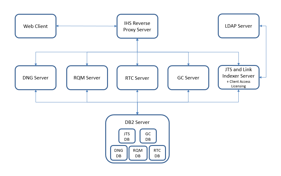
Test Topology
The specific versions of software used were:
| Software |
Version |
|---|---|
| IBM Rational CLM Applications |
6.0 |
| IBM HTTP Server and Web Server Plugin for WebSphere |
8.5.5.2 |
| IBM WebSphere Application Server |
8.5.5.1 |
| IBM Tivoli Directory Server |
6.1 |
| DB2 Database |
10.5 |
Test Machine Details
| Function | Number of Machines | Machine Type | CPU / Machine | Total # of CPU cores | Memory/Machine | Disk | Disk capacity | Network interface | OS and Version |
|---|---|---|---|---|---|---|---|---|---|
| Reverse Proxy Server (IBM HTTP Server and WebSphere Plugin) | 1 | IBM x3250 M3 | 1 x Intel Xeon CPU X3480 3.07GHz (quad-core) | 4 | 15.5GB | RAID 0 -- SAS Disk x 1 | 279GB | Gigabit Ethernet | Red Hat Enterprise Linux Server release 6.6 (Santiago) |
| JTS/LDX Server | 1 | VM image | n/a | 8 vCPU | 32GB | SCSI (virtual) | 80GB | virtual | Red Hat Enterprise Linux Server release 6.6 (Santiago) |
| GC Server | 1 | VM image | n/a | 8 vCPU | 32GB | SCSI (virtual) | 80GB | virtual | Red Hat Enterprise Linux Server release 6.6 (Santiago) |
| RQM Server | 1 | VM image | n/a | 8 vCPU | 32GB | SCSI (virtual) | 80GB | virtual | Red Hat Enterprise Linux Server release 6.6 (Santiago) |
| RTC Server | 1 | VM image | n/a | 8 vCPU | 32GB | SCSI (virtual) | 80GB | virtual | Red Hat Enterprise Linux Server release 6.6 (Santiago) |
| DNG Server | 1 | VM image | n/a | 8 vCPU | 32GB | SCSI (virtual) | 80GB | virtual | Red Hat Enterprise Linux Server release 6.6 (Santiago) |
| DB2 Server | 1 | IBM x3650 M3 | 2 x Intel Xeon CPU X5667 (quad-core) | 8 | 31.3GB | RAID 10 -- SAS Disk x 8 | 279GB | Gigabit Ethernet | Red Hat Enterprise Linux Server release 6.6 (Santiago) |
The Global Configuration Service
A global configuration is a new concept in the 6.0 release that allows you to assemble a hierarchy of streams or baselines from domain tools such as DNG, RQM, and RTC. You use a global configuration to work in a unified context that delivers the right versions of artifacts as you work in each tool, and navigate from tool to tool. This capability is delivered by a new web application (the global configuration application). Our performance testing for 6.0 looked at the following aspects of the global configuration (gc) application:- What was the maximum throughput for the gc application?
- For the GC web UI
- For the requests issued to the GC app from the other applications
- How much memory and CPU does the gc application consume at different load levels?
- For the GC web UI
- For the requests issued to the GC app from the other applications
- How do the CLM applications (RQM, DNG, RTC) interact with the gc application? At what point does the gc application become a bottleneck?
Performance of the Global configuration Web UI
This set of tests focused on the behavior of the Web UI for the global configuration application. The Web UI is used to manage global configurations (creating streams and baselines, associating streams and baselines from other applications with global configurations, creating components and searching). The Web UI would typically be used by a small percentage of the user population, since it is used for release management functions which most people won't need to carry out. Most people interact with global configurations indirectly, through the user interfaces of the applications like RQM or DNG.We carried out these tests by first developing automation that would simulate users interacting with the GC web UI. We then executed the simulation while incrementally increasing the user load, watching for the point at which the transaction response times started to increase. We watched the CPU utilization for the different servers in the test topology to see how this varied as the throughput increased. This is a summary of what we found.
- Response times started to increase when the workload exceeded 1100 simulated users. The throughput handled by the GC application at this load was 107 requests per second.
- The CPU utilization of the GC application was relatively low (21%) at this point. The limiting factor was actually the DNG server, which reached 76% CPU utilization at 1100 users. This happened because process of creating GC streams and baselines involves interactions with the other application servers (to look up local configurations). The GC application was actually capable of handling more transactions that we could simulate in this test.
- We can extrapolate the limits of the GC application, and estimate that the maximum throughput would be 455 transactions per second, and at that rate, the CPU utilization for the GC application would reach 83%. Although the test topology could not reach these levels because of application bottlenecks, topologies involving multiple application servers or federated CLM deployments could drive a GC application at an equivalent of 4675 users (creating 10,625 streams and baselines per hour, while searching/browsing 599,000 times an hour).
Workload characterization
| User Grouping | Percentage of the workload | Use Case | Use Case Description |
|---|---|---|---|
| Reads | 70% | ListComponentsPaged | Search for the first 25 global components. Results returned in one page. |
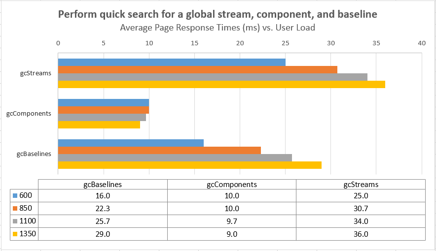
| QuickSearch | Search for a global stream, component, and baseline (in that order). | ||
| SearchAndSelectComponent | Search for a global component and click link to view component details. | ||
| Writes | 30% | CreateAndCommitBaseline | Search for a global stream configuration for a specific component, use the stream configuration to create a staging area for global baseline creation, replace the contributing stream configurations for DNG and RQM with a baseline configuration, replace the contributing stream configuration for RTC with a snaphot, and commit the global baseline. |
| CreateStreamFromBaseline | Search for a global baseline for a specific component, use the baseline configuration to a create a global stream, replace the contributing baseline configurations for DNG and RQM with a stream configuration, and replace the contributing snapshot for RTC with a stream configuration. |
Data shape and volume
Here is the initial size of the repository:- 131 global components
- 131 linked application projects (e.g. 131 RQM, RTC, and DNG projects)
- 131 global streams
- 262 global baselines
- GC database size = 807M
Results
Response times for operations as a function of user load
The charts below show the response times for the different use cases in the workload as a function of the number of simulated users. There is a sharp increase in many response times at the 1350 user level; the response times are relatively flat up to 1100 users. Based on these results, we use the 1100 user level as the maximum supportable workload for this test topology. Note that many of the operations which have degraded involve interaction with the applications. For example, the rmSelectRandomBaseline operation is measuring the response time of the DNG server. Search or list operations in the GC UI remain fast even at 1350 users.
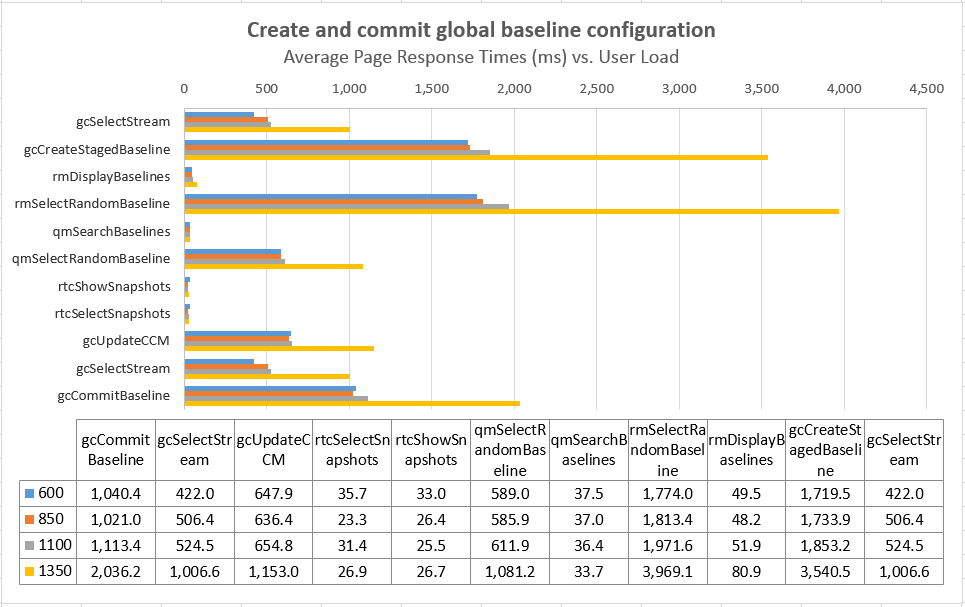
Average Page Response Times vs User Load Comparisons
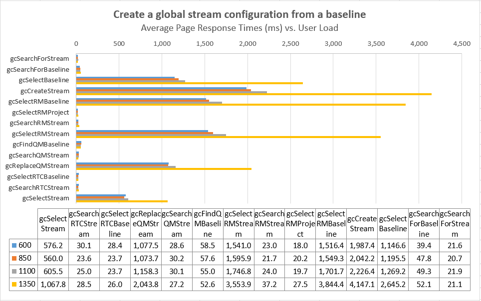
Average Page Response Times vs User Load Comparisons
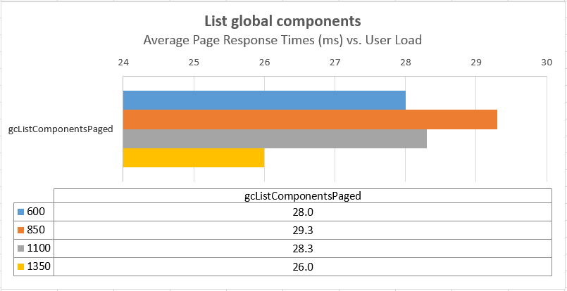
Average Page Response Times vs User Load Comparisons
Average Page Response Times vs User Load Comparisons
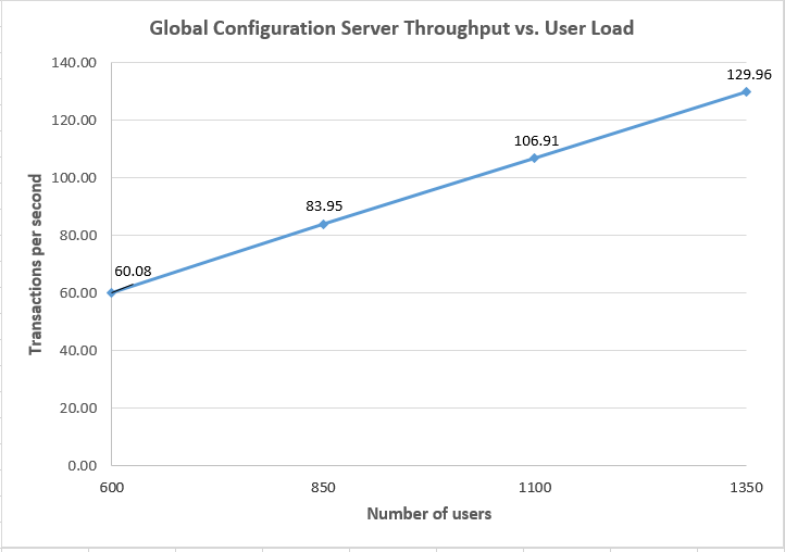
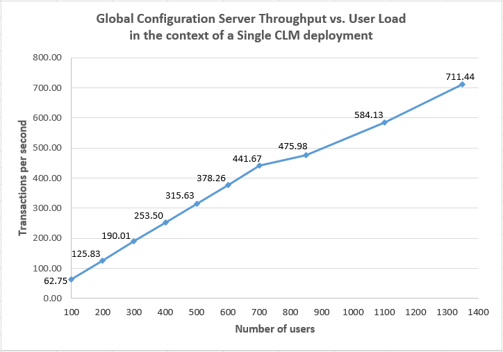
Throughput as a function of user load
This chart shows how many transactions per second were processed by the GC application at different user loads.
Throughput vs User Load Comparisons
CPU utilization vs. transaction rates
This chart looks at the CPU utilizations for the different servers in the test topology, as a function of GC throughput. Note that the DNG server is near its CPU limit at 130 transactions per second, which suggests that the DNG server is the bottleneck for this particular workload. The GC application is only at 24% CPU; it is capable of processing more requests.

Average CPU vs Throughput Comparisons
Estimated maximum throughput
Given that the GC application did not reach its maximum, we used the available data to estimate the point at which the GC application would become overloaded. Here we assume that CPU would be the limiting factor, and that the GC application will behave linearly as the load increases. The chart below extends the CPU data to higher throughput levels, and from this we can estimate that the GC application is actually capable of processing 455 transactions per second (at which point the CPU utilization would be 83%).
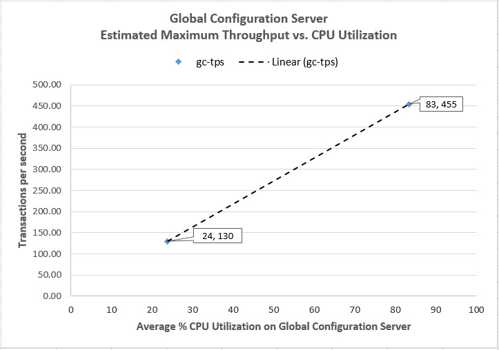
Projected Maximum Throughput for Global Configuration as a Standalone Application
The table below describes the limits of the GC application from higher-level perspective. We derive the estimate maximums by using the ratio between the estimated maximum throughput (455) and the actual throughput at 1100 users (107). We multiple the values measured at 1100 users by this ratio (4.25) to estimate the maximum values.
| Name | Measured value | Maximum (estimated) |
|---|---|---|
| # Users | 1100 users | 4675 |
| Rate of stream, baseline creation | 2500 per hour | 10625 per hour |
| Rate of search/browse | 141,000 | 599,000 |
| GC transactions per second | 107 | 455 |
Global Configuration performance in the context of a single Jazz instance
Now we look at the behavior of the GC application when used in typical integration scenarios, such as creating links between a work item and a test case, or a test case and a requirement, or a work item and a requirement. These scenarios involve users interacting with the UIs of RTC, RQM, and DNG - the users don't interact directly with the GC Web UI. In these scenarios, there are two primary ways in which the GC application is used:- Searching for GC streams or baselines when selecting a global configuration in RQM or DNG
- Resolving local configurations from global configurations
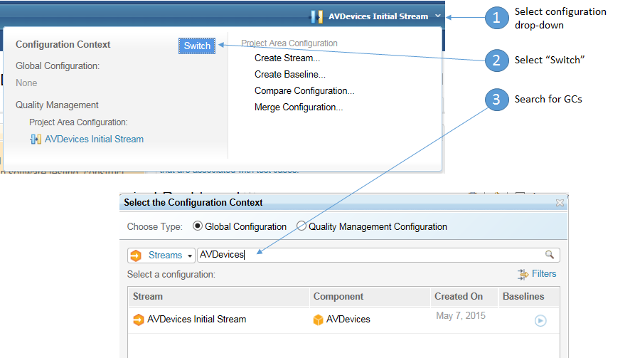
Selecting a global configuration
GET /gc/configuration/<id>This tells the applications which local streams or baselines correspond to the global stream or baseline. We've previously looked at how the GC app handles searching. In this next set of tests, we first look at how well the GC application can resolve global configurations to local configurations. Then, we look at an integration scenario to see how much stress DNG, RTC, and RQM place on the GC application.
Workload characterization
The GC simulation workload was designed to artificially stress the capability of the GC application to provide the local configurations that are associated with global configurations. The automation searches for a global configuration, and then issues a number of GET requests to retrieve the local configurations associated with the global configuration. The ratio of GET requests to search requests in this artificial workload is 7:1. Test results for this workload start in this section.| User Grouping | Percentage of the workload | Use Case | Use Case Description |
|---|---|---|---|
| GC Simulation | 100% | QM_OSLCSim | Request global configuration via RQM proxy. |
| RM_OSLCSim | Request global configuration via DNG proxy. |
- The selection of global configurations involves sending search requests to the GC app, followed by GET requests to resolve of the global configuration to local configurations.
- Artifact linking involves GET requests to resolve a global configuration to local configurations (with potential caching of the local configuration to avoid extra calls to the GC app)
| User Grouping | Percentage of the workload | Use Case | Use Case Description |
|---|---|---|---|
| RTC-DNG Integration | 31% | LinkDefectToRequirement | Open a new defect, set 'Filed Against' field to current project and 'Found In' field to the release which corresponds to global configuration, save defect, click Links tab, click to add link type 'Implements Requirement', select to create a new requirement, input requirement information and save requirement, and save defect. |
| RTC-RQM Integration | 31% | LinkDefectToTestCase | Open a new defect, set 'Filed Against' field to current project and 'Found In' field to the release which corresponds to global configuration, save defect, click Links tab, click to add link type 'Tested by Test Case', select to create a new test case, input test case information and save test case, and save defect. |
| RQM-DNG Integration | 31% | LinkTestCaseToRequirement | In the context of a global stream configuration, open a new test case, input test case information and save, click Requirements tab, click to create a new requirement, input information and save requirement, and save test case. |
| GC Selections | 7% (50/50) | QMSelectGlobalConfiguration | Resolve the local configuration context for RQM by searching for and selecting a specific global stream configuration. |
| RMSelectGlobalConfiguration | Resolve the local configuration context for DNG by searching for and selecting a specific global stream configuration. |
Stress testing the GC application
The tests described in this section simulate the interactions of the CLM applications with the GC application, but the simulation is designed to artificially stress the GC application in order to estimate its maximum throughput. We can then compare this maximum throughput to that observed in normal usage in order to estimate how much link creation a single GC application can support. The simulations issue requests for global configuration URIs to the DNG or RQM applications. DNG and RQM then send messages to the JTS to authenticate and then finally these applications forward the request to the GC application. In our test topology where the GC, DNG, JTS, and RQM applications are all on separate servers (with a reverse proxy on the front-end), this interchange involves cross-server network communication.Summary of results
In this test, we slowly increased the number of simulated users requesting information about global configurations, and we looked at the response times, CPU utilization, and throughput for the various servers in the test topology. Here's what we found.- The performance of the system begins to degrade above 700 simulated users. It becomes increasingly difficult to push transactions through the system, and the throughput flattens out around 1350 simulated users.
- At 700 users and below, the response times are not sensitive to load, and so the throughput increases linearly as the number of simulated users increases.
- The GC and the JTS server have the highest CPU utilization (in the 60-70% range at 1350 users)
- The response times for transactions sent directly to the GC application are not strongly impacted by the increasing load. More time is spent within the RQM and DNG applications, on these calls:
- In RQM: calling the service to translate a global configuration to local configuration
- In RQM: getting the default global configuration
- In RQM: retrieving a global configuration URI from the GC application (qm/proxy)
- In DNG: retrieving a global configuration URI from the GC application (rm/proxy)
Detailed results
This chart shows how the throughput processed by the GC application varies as the simulated user load increased. The throughput increases linearly up to the 700 user level, at which point it begins to fall off as the other applications start to struggle.
Throughput vs User Load Comparisons
This chart shows how the CPU utilization of the test servers changes as the user load increases. Above 1400 simulated users, the CPU usage flattens out. This happens because the servers are struggling to process the load, and the response times are increasing as a consequence of that struggle. Because the transactions are taking longer to process, the throughput flattens out, and so the CPU usage flattens out as well.
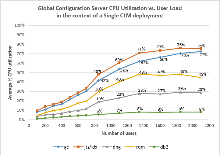
Average CPU vs User Load Comparisons
This chart is an alternative view, showing the CPU utilization as a function of the throughput handled by the GC application.
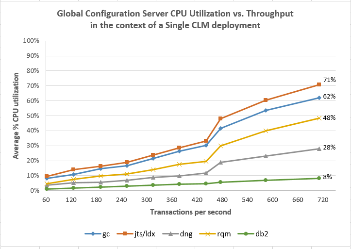
Average CPU vs Throughput Comparisons
This chart shows the response times for the transactions that are part of the simulation.
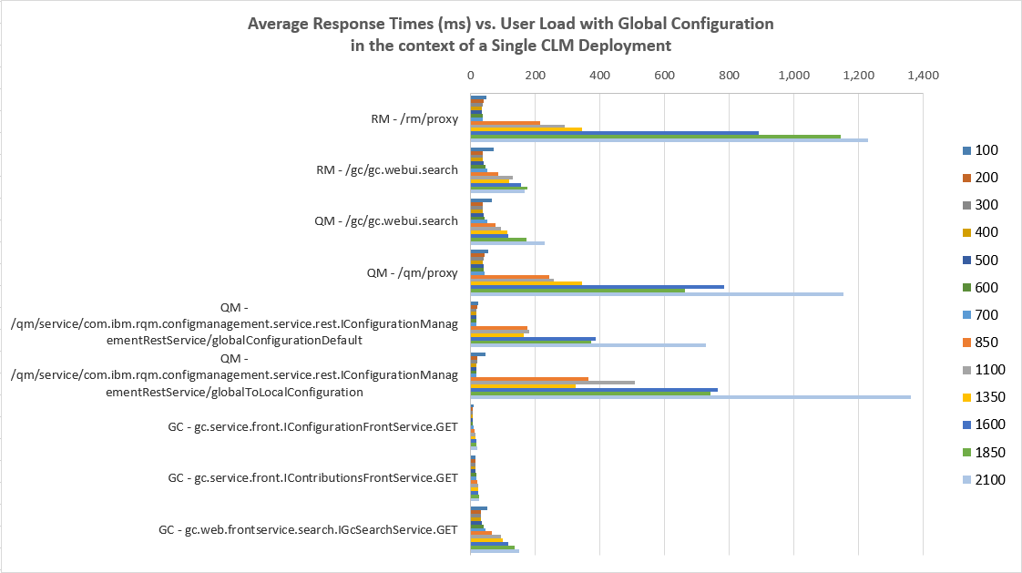
Average Response Times vs User Load Comparisons
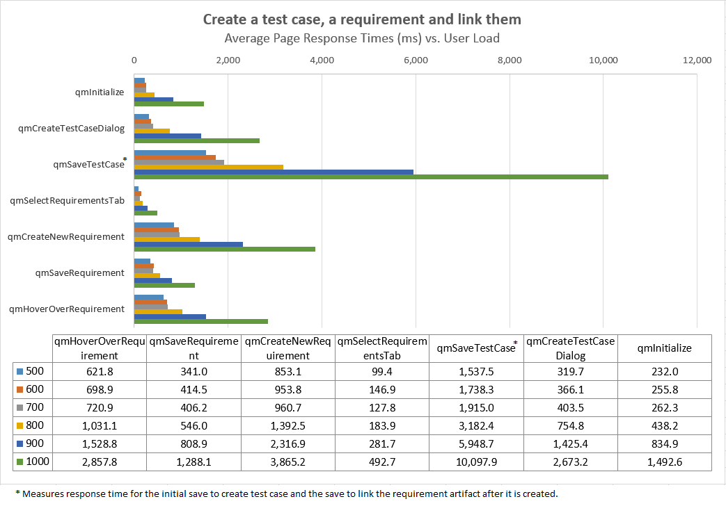
Results for the integration scenario
Here are the results for the simulation of the integration scenario.- The system supported a maximum of 1000 users (although response times at this level were degraded). At this point, the CPU utilization of the RQM server had risen to 100% (and the DNG and RTC servers were also extremely busy).
- The CPU utilization in the GC application was low (.4%), and the number of transactions per second processed by the GC application was low (.53 per second) compared to its maximum throughput.
- The response times for the integration use cases were flat through 700 users, but started to degrade at 800 users and up.
10326 links per hour x (316 TPS maximum / .53 TPS at 10326 links per hour = 6.2 million links per hourA single CLM deployment would not be able to achieve this rate. But you can use this rate as the upper limit for a more complex, federated deployment where there are multiple independent CLM instances (each with their own JTS), all sharing a centralized deployment of the GC application.
Link creation rates for the integration workload
| Integration Scenario | Number of links created per hour vs. User Load | |||||
|---|---|---|---|---|---|---|
| 500 | 600 | 700 | 800 | 900 | 1000 | |
| RTC-DNG | 1,664 | 2,018 | 2,360 | 2,697 | 2,949 | 3,205 |
| RTC-RQM | 1,659 | 2,010 | 2,356 | 2,611 | 2,881 | 3,053 |
| RQM-DNG | 2,277 | 2,728 | 3,143 | 3,540 | 3,838 | 4,068 |
CPU Utilization as a function of user load
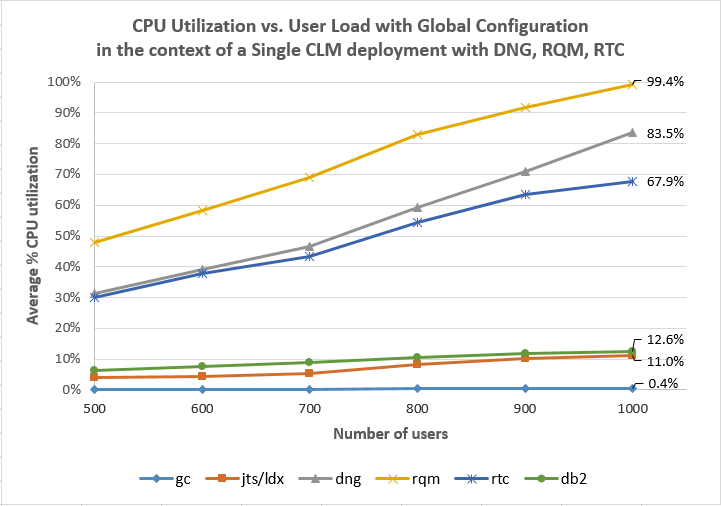
Average CPU vs User Load Comparisons
Throughput as a function of user load
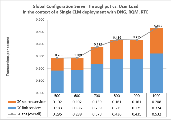
Throughput vs User Load Comparisons
Response Time summaries
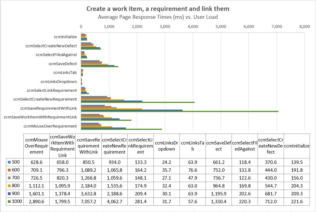
Average Page Response Times vs User Load Comparisons
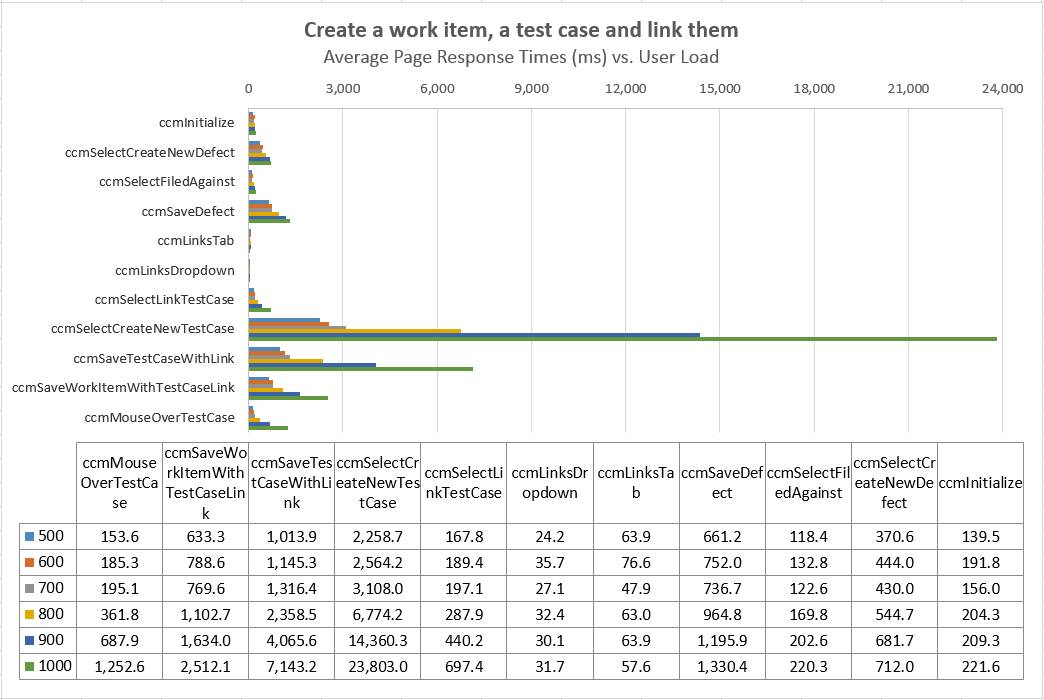
Average Page Response Times vs User Load Comparisons
Average Page Response Times vs User Load Comparisons
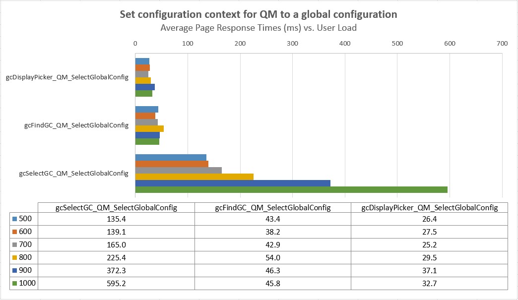
Average Page Response Times vs User Load Comparisons
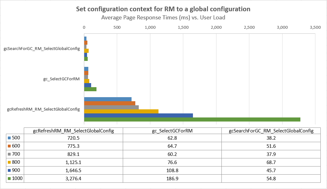
Average Page Response Times vs User Load Comparisons
The Link Indexing Service (LDX)
The link indexing service keeps track of the links between versions of artifacts. The service is deployed as a separate web application, and will poll every minute to pick up changes in Rational Team Concert, global configurations or Rational Quality Manager. If links are created between artifacts, the back link service will store information about the two linked artifacts and the kind of link relating them. Later on, applications can query the back link service to determine what links are pointing back at a particular artifact. If you open the Links tab in a requirement, the back link service will provide information about any work items or test artifacts that reference the requirement. If you open a test artifact, the back link service will provide information about what work items or release plans reference the test artifact. Our testing of the link service looked at the following things:- The maximum rate at which the back link service could process changes from RQM or RTC
- The CPU utilization of the link service
- The time required to create the initial index, when enabling configuration management
- The disk space required to store the link index
Initial indexing performance after enabling configuration management
When you first deploy the 6.0 release, the configuration management features are not enabled, and the back link indexing service is not active. To enable configuration management, you must specify an activation key in the Advanced Properties UI for your RQM and DOORS Next Generation services. When you enter the activation key for Rational Quality Management, the system will automatically locate your Rational Team Concert and Rational Quality Manager data and begin indexing all of your project areas. This may be a lengthy process, but you can continue to use your project areas while the indexing process is going on. In our testing, we found that the initial indexing could proceed at the following rates:- 75.9 work items per second
- 64.2 test cases per second
| Application | Artifact count | Time required |
|---|---|---|
| Rational Team Concert | 223843 | 49m 8s |
| Rational Quality Manager | 437959 | 1hr 53m 36s |
Link indexing during integration scenarios
In this set of tests, we looked at 3 common integration scenarios, to see how fast the link indexer could process changes. The scenarios were:- Creating a new test case and a new requirement, then creating a link from the test case to the requirement
- Creating a new work item and a new requirement, then creating a link from the work item to the requirement
- Creating a new work item and a new test case, then creating a link form the work item to the test case
- The CPU used by the link indexer is low, even at high loads. The CPU utilization increases slightly as load increases, but the highest utilization we observed was only 4.3%
- For this test topology, the bottlenecks are in the applications. It is harder to do the work of creating new artifacts and linking them together than it is to update the link index. Even with an artificial workload intended to stress the LDX, we could not create links fast enough to overload the LDX.
- The LDX can process work items at a maximum rate between 50 and 60 work items per second.
- The LDX can process test cases at roughly a maximum rate of 20 test cases per second (when links are being created from work items to test cases). This rate drops to 10 per second if links are being created from the RQM side.
- For linking work items to requirements: 198000 links per hour (assuming 55 links per second)
- For linking test cases to requirements: 36000 links per hour
- For linking work items to test cases: 72000 links per hour (RQM processing rate of 20 per second is the limiting factor)
Detailed results from link indexing tests
This section provides the details from the tests of link indexing performance. We conducted these tests by simulating the behavior of users that were creating pairs of new artifacts and then linking them together. We increased the number of simulated users until we encountered a bottleneck somewhere in the system. During the test, we monitored the link indexing application to extract out information about the number of changes it processed per second. We also watched the link indexer to make sure it was keeping up with the incoming traffic and not falling behind. The table below summarizes the rates at which the automation could create links at the different user loads.| Integration Scenario | Number of links created per hour vs. User Load | ||||||||
|---|---|---|---|---|---|---|---|---|---|
| 30 | 60 | 90 | 120 | 150 | 180 | 210 | 240 | 270 | |
| RTC-DNG | 3,492 | 6,936 | 10,416 | 13,792 | 17,232 | 20,496 | 23,600 | 26,156 | 29,140 |
| RTC-RQM | 3,488 | 6,984 | 10,484 | 13,972 | 17,452 | 20,884 | 24,440 | 27,944 | 31,280 |
| RQM-DNG | 3,324 | 6,656 | 9,908 | 13,188 | 16,080 | -- | -- | -- | -- |
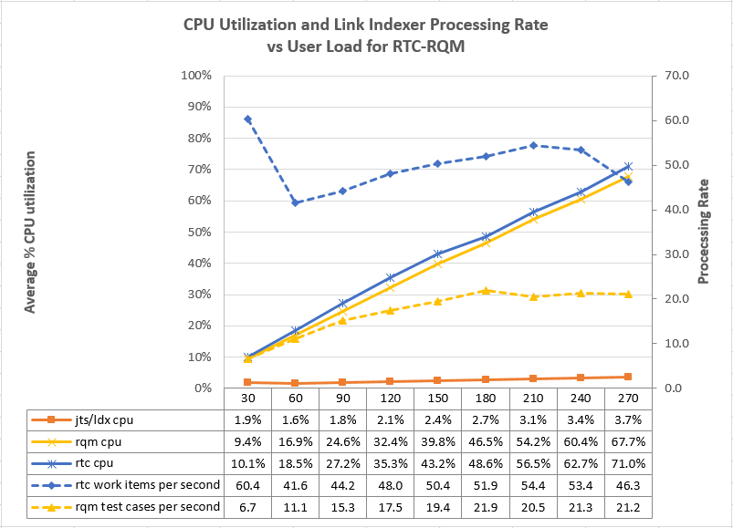
Linking work items to requirements
This test simulated a collection of users that were linking work items to requirements. The automation simulated the following operations:
- Create a new work item and save it
- From the work item links tab, select "Add Implements Requirement"
- Select the "Create New" option. Fill in the "New requirement" dialog and save the requirement
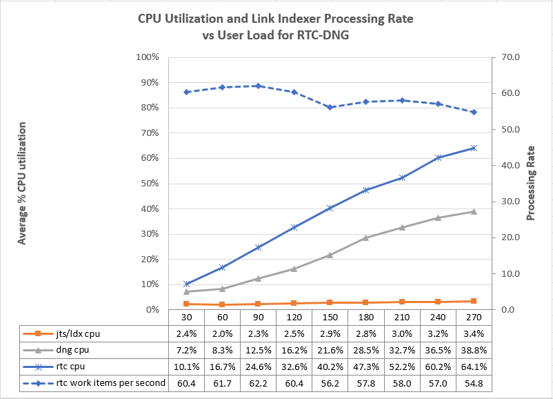
Average CPU and Processing Rate vs User Load
Linking work items to test cases
This test simulated a collection of users that were linking work items to test cases. The automation simulated the following operations: - Create a new work item and save it
- From the work item links tab, select "Add Tested by Test case"
- Select the "Create New" option. Fill in the "New Test case" dialog and save the test case
Average CPU and Processing Rate vs User Load
Linking test cases to requirements
This test simulated a collection of users that were linking test cases to requirements. The automation simulated the following operations:
- Create a new test case and save it
- Open the test case and select "Requirement Links"
- Select the "Create New Requirement" option. Fill in the "New Requirement" dialog and save the requirement
- Save the test case
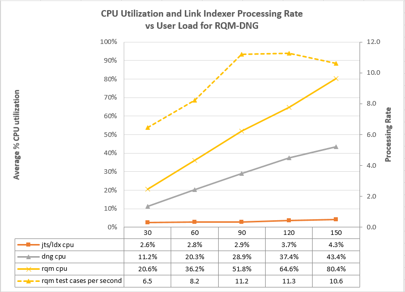
Average CPU and Processing Rate vs User Load
Appendix A: System parameters/tunings
WebSphere Application Servers
We set the LTPA token timeout in WebSphere artificially high on all servers because our test automation logs in once, and then reuses the credentials for the duration of the test. Setting the timeout to a high value prevents the credentials from becoming invalid in long test runs. We do not recommend using this setting in production systems. When credentials time out in production systems, clients are prompted to re-authenticate. Our performance automation is not sophisticated enough to re-authenticate.JTS/LDX
Increased WebContainer thread pool min/max settings to 200/200Increased LTPA token timeout to 12000
Increased application JDBC and RDB mediator pool sizes to 400
JVM arguments were set to:
-Xgcpolicy:gencon -Xmx16g -Xms16g -Xmn4g -Xcompressedrefs -Xgc:preferredHeapBase=0x100000000 -XX:MaxDirectMemorySize=1G -Xverbosegclog:logs/garbColl.log
GC
Increased WebContainer thread pool min/max settings to 400/400Increased LTPA token timeout to 12000
Increased application JDBC and RDB mediator pool sizes to 400
JVM arguments were set to:
-Xgcpolicy:gencon -Xmx16g -Xms16g -Xmn4g -Xcompressedrefs -Xgc:preferredHeapBase=0x100000000 -XX:MaxDirectMemorySize=1G -Xverbosegclog:logs/garbColl.log
DNG, RQM, RTC
Increased WebContainer thread pool min/max settings to 400/400Increased LTPA token timeout to 12000
Increased application JDBC and RDB mediator pool sizes to 400
JVM arguments were set to:
-Xgcpolicy:gencon -Xmx24g -Xms24g -Xmn6g -Xcompressedrefs -Xgc:preferredHeapBase=0x100000000 -XX:MaxDirectMemorySize=1G -Xverbosegclog:logs/garbColl.log
IBM HTTP Server
In httpd.conf:
<IfModule worker.c>
      ThreadLimit           25
      ServerLimit           80
      StartServers          1
      MaxClients            2000
      MinSpareThreads       25
      MaxSpareThreads       75
      ThreadsPerChild       25
      MaxRequestsPerChild   0
</IfModule>
Appendix B: Overview of the internals of the link indexing service
The link indexing service is meant to run behind the scenes. It is automatically configured and used by the CLM application, so under normal conditions, you don't even need to know it is there. Still, a brief overview of the implementation of the link indexing service may help to put some of the test results into context. The first thing to know is that changes made to work items, global configurations, and test artifacts are tracked by the applications and exposed by each application as a "tracked resource set" (also known as a TRS feed). From the perspective of the LDX, each TRS feed is considered a "data source". The LDX polls the data sources looking for new changes once per minute; there will be one data source per application per server. In our test topology, for example, the LDX knows about three data sources: one for the RQM server, one for the RTC server, and one for the GC server. Since the integration scenarios did not involve GC creation, there is no indexing activity for the GC data source in these tests.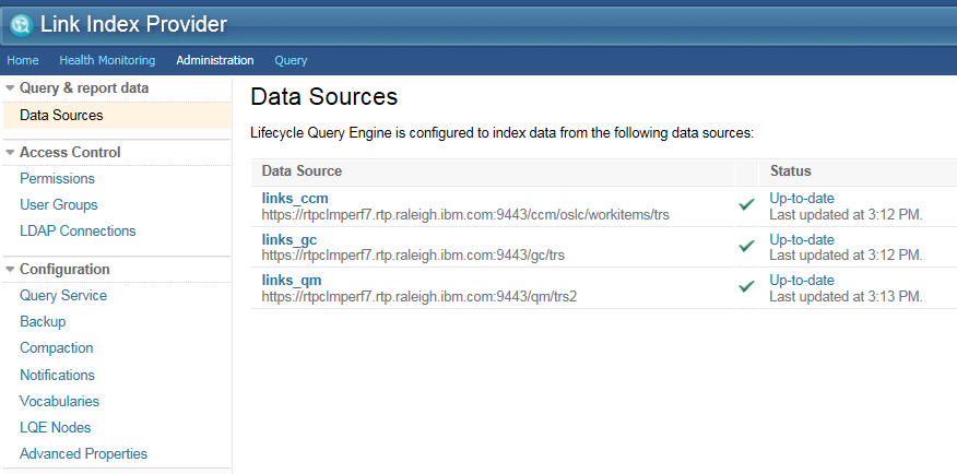
Deployments that have more servers will have more data sources, and the LDX will cycle through all of the data sources it knows about once per minute. When it wakes up, it retrieves the list of changes since the last time it checked. It then gets details about each of the changed artifacts, and updates the link index if it finds that a link has been added. The next thing to know is that each data source will be processed by 2 threads (by default, although this can be configured). This has two implications:
- There is a limit on the amount of CPU that an LDX will consume, which is determined by the total number of data sources and the number of threads per data source
- As more data sources are added, there is a potential for additional threads to run, and for the LDX to become busier.
How we measured link indexing rates
This section describes how we estimated the maximum processing rates for the LDX, as described in this section.The LDX runs behind the scenes and does not normally require attention. It does, however, have a rich set of administration features (accessible via the ldx/web URL), and we used these features to get an idea of what the LDX was doing when the CLM system was under load. If particular, if you drill down into the status of the data sources, you can find a History tab which summarizes past indexing activity, and the "View change log" link provides detailed information about what happened during each LDX polling interval.
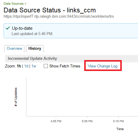
LDX admin UI: data source status
The information provided by the change log is shown below, for a single load level for each of the scenarios. The key bits of information are:
- the "Retrieved" column, which is the number of artifacts processed from the data source in the last polling interval
- the Duration column, which is the total time in seconds which the LDX spent processing those artifacts
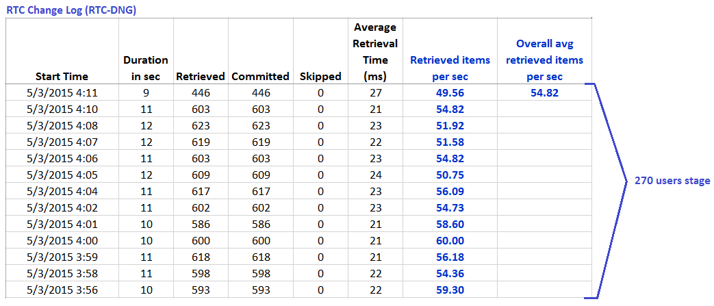
RTC Change Log data reported for RTC-DNG links created during 270 users stage
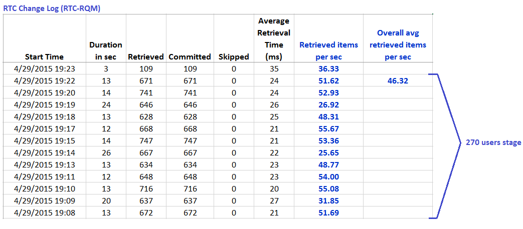
RTC Change Log data reported for RTC-RQM links created during 270 users stage
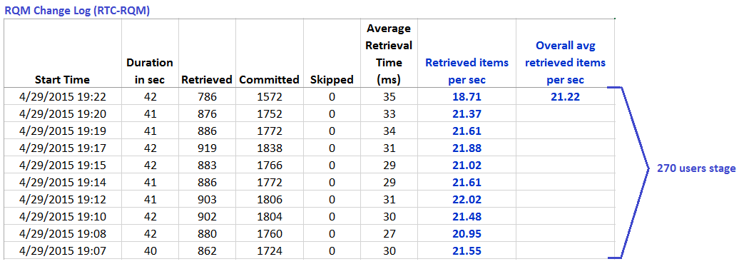
RQM Change Log data reported for RTC-RQM links created during 270 users stage
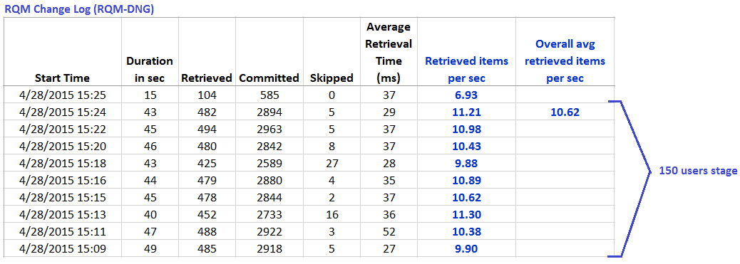
RQM Change Log data reported for RQM-DNG links created during 150 users stage
Related Information
Contributions are governed by our Terms of Use. Please read the following disclaimer.
Dashboards and work items are no longer publicly available, so some links may be invalid. We now provide similar information through other means. Learn more here.