Rational DOORS Next Generation: Organizing requirements for best performance
Author: VaughnRokoszBuild basis: 6.x
General observations on DNG performance
Before we get to the details on data limits, it would be helpful to review how DNG stores data, and to look at areas where data growth can lead to performance degradation (and why). If you aren't interested in the details, feel free to skip ahead to the next section Ways of organizing requirements. The first thing to know is that DNG keeps data in two places:- In a relational database on a database server (Oracle, DB2, SQL Server). There are a number of database tables and indices that support DNG; these are updated when artifacts are created, modified, or deleted and are often read when artifacts are queried.
- In files local to the DNG server. These local files are intended to speed up queries. They contain two sorts of data:
- A full-text index which supports searching for artifacts that contain text keywords. The technology that supports full-text indexing is based on Lucene; the default location of the full-text index is under server/conf/rm/indices/workitemindex.
- Information about the relationships between artifacts based on the Resource Description Framework (RDF) standard. The technology that supports RDF is Jena; the default location of the Jena index is under server/conf/rm/indices/
/jfs-rdfindex.
Performance issues in the relational database
As a DNG repository grows, the number of records in the relational tables will also grow. For example, there is a table that has an row for each version of an artifact. If you have 1 million artifacts and you've created 3 versions of each artifact, your version table will have 3 million rows. The database vendors usually do a good job of optimizing SQL queries so that they can efficiently extract data from large databases (by using indices, for example). But having a large number of artifacts can mean that your queries will be returning more data, and if that happens, performance can degrade. If a project area gets too big, then SQL queries that are scoped to a project area may have to do full table scans rather than use indices. If a DNG module gets too large, the SQL statements that retrieve the artifacts that are in a module can slow down. The SQL for module queries is especially problematic on Oracle. You can mitigate these issues by taking the following actions:- Keep your database statistics updated as the repository grows. This will allow the SQL optimizers to do a better job, since they'll make decisions based on the current sizes.
- If you are using Oracle Enterprise, you can run the SQL Advisor to further optimize SQL. Oracle can sometimes recommend improved access plans for executing SQL.
- Oracle also allows you to move database tables and views into a KEEP buffer pool, to cache frequently used data for longer. You can use the SQL Advisor to identify common or expensive SQL statements, and move the tables and views from those statements into the KEEP buffer pool.
- You can increase the amount of memory used by the database server, which will allow more data to be cached in memory.
exec dbms_stats.delete_column_stats(ownname=>'RM', tabname=>'VVCMODEL_VERSION', colname=>'CONCEPT', col_stat_type=>'HISTOGRAM');
exec dbms_stats.delete_column_stats(ownname=>'RM', tabname=>'VVCMODEL_VERSION', colname=>'STORAGE', col_stat_type=>'HISTOGRAM');
exec dbms_stats.delete_column_stats(ownname=>'RM', tabname=>'VVCMODEL_VERSION', colname=>'VERSION', col_stat_type=>'HISTOGRAM');
exec dbms_stats.set_table_prefs('RM', 'VVCMODEL_VERSION', 'METHOD_OPT', 'FOR ALL COLUMNS SIZE AUTO, FOR COLUMNS SIZE 1 CONCEPT, FOR COLUMNS SIZE 1 STORAGE, FOR COLUMNS SIZE 1 VERSION');
exec dbms_stats.gather_table_stats (OWNNAME=>'RM', TABNAME=> 'VVCMODEL_VERSION');
#RDFPerformance
Performance issues in the RDF (Jena) index
The Jena index is stored locally on the DNG server, and contains information about the relationships between artifacts. There are many different kinds of relationships (links, containment, comments) and so this index can get large as the number of artifacts grows. For example: in IBM tests, a repository with 2 million artifacts results in a Jena index that takes 157G of disk space. As of the 6.0.2 release, DNG uses memory-mapped filesto access Jena data (at least on Linux). Jena files are mapped into the address space of the DNG Java process, and then are brought into memory by the operating system and stored in the page cache. Accessing pages that are already in memory will be fast. If DNG needs to access Jena data that is not in memory, the operating system will generate a page fault and then read the data into memory from disk. Updates to DNG data will write to the page cache, marking the pages as "dirty" - and dirty pages are periodically flushed back out to disk. Prior to 6.0.2, DNG relied more heavily on the Java heap for Jena data; the move to memory-mapped I/O reduced the amount of heap required significantly, which in turn allowed larger repositories to be supported.Note: Memory-mapped I/O is not enabled by default for Windows, since there have been problems reported when using memory-mapped I/O on Windows virtual systems. We recommend that you use Linux as your operating system, if at all possible.The operating system uses any available RAM for the page cache, but will automatically shrink or grow the page cache based on the memory demands of other applications. On Linux, you can get information about the size of the page cache by running "free -m":
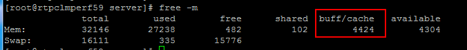 In this example - the server has 32G of total RAM, and 27G are being used by applications running on the server. The bulk of that application memory is the DNG server itself - on this system, the JVM has a 22G heap. The page cache is 4424M in size - so this is how much memory is available for caching Jena data. But keep in mind that the page cache will shrink if other applications need memory. If the page cache is small relative to the size of the Jena index, then the DNG server will read data from disk more frequently, and that will be slower.
This all has several important implications for performance:
In this example - the server has 32G of total RAM, and 27G are being used by applications running on the server. The bulk of that application memory is the DNG server itself - on this system, the JVM has a 22G heap. The page cache is 4424M in size - so this is how much memory is available for caching Jena data. But keep in mind that the page cache will shrink if other applications need memory. If the page cache is small relative to the size of the Jena index, then the DNG server will read data from disk more frequently, and that will be slower.
This all has several important implications for performance: - You can improve DNG performance by adding RAM, because this allows the page cache to be bigger. To be conservative, add the JVM heap size to the Jena index size on disk, and use that number as the amount of RAM for the DNG server. For example, if you have a 16G JVM heap and a Jena index size of 22G - you should have 38G or more of RAM on your DNG server - that will allow for most of the Jena index to be cached in memory.
- You can improve DNG performance by using the fastest possible disk drives (like SSD drives). A fast disk drive will reduce the performance penalty of a page fault, so that reading Jena data into memory will not be as costly. As importantly, flushing the page cache out to disk will also be faster, so that DNG write operations will be faster with faster disk i/o.
- Avoid oversizing your JVM. Memory used by the JVM is not available to the page cache, so the bigger your JVM heap size is, the less memory will be available for caching the Jena data. Use verbose gc logging and tools like IBM's GCMV to base your sizing decisions on the heap usage from your workload.
Performance issues in the full-text index
Full-text searches are scoped by project area, and then results are filtered. For example, if you create a module view that involves a full-text search, it will look across the entire project area for candidates and then filter the hits down to those that are specific to the module. What that means is that as the project area grows in size, the number of potential hits can grow. If you search on a common keyword, you can end up with tens of thousands of candidates. The cost to filter out the hits that don't apply can be high - a search that returns 85,000 candidates can take 5 minutes or more.Caching
The final performance topic concerns caches. DNG keeps recently-accessed data in memory. If a DNG user is working with artifacts that are cached, performance is better than if the data is not yet cached. In some cases, having data in a cache avoids SQL calls altogether, which reduces load on the database server. On the other hand, when data is not yet cached, there is a performance penalty for the first person that accesses an artifact. As a DNG repository grows in size, or as the complexity of artifacts grows, that penalty can become severe (minutes). Immediately after a server restart, the caches are empty, and so response times will be higher initially until the system warms up and the caches become populated. Once the system reaches a steady state, the caches should be populated with frequently used artifacts, and most users should see good performance. A few users may see poor performance when accessing data that isn't cached. That concludes my review of factors influencing DNG performance. Now, I'll move on to the features available for organizing requirements, and the known limits on artifact counts.Ways of organizing requirements
DNG provides a number of ways of organizing your data. While there are no hard limits, there are practical limits as to how big your DNG systems can get and these practical limits are not independent of each other. For example, there are limits on both the total number of artifacts in a server, and the total number of artifacts in a project area. That means you need to split up your requirements across several project areas as the repository grows in size. Also keep in mind that if you are planning to push the limits for the DNG server overall, or for a single project area, then you will need to use the fastest disk drives available (like SSD). You should also use Linux as the operating system for the DNG server, and DB2 as the database. While we don't have extensive data comparing Linux/DB2 systems to Windows/Oracle systems, we do know that the data scale can be reduced as much as 50% on virtual Windows systems. And we know that module loading can be slow on Oracle. The table below lists the options available for organizing data and summarizes the practical limits for each:|
Feature |
Limitations |
|
DNG server |
2,000,000 total requirements (or 20M versions if configuration management is enabled) |
|
Number of DNG servers |
No known limits. 15 or more per JTS have been successfully deployed in the field. |
|
Project area |
200,000 artifacts |
|
Component |
100 components per project area |
|
Module |
10,000 artifacts per module |
|
Folder and folder hierarchy |
10,000 artifacts per folder; avoid flat folder hierarchies |
|
Views and queries |
10,000 artifacts returned |
Folders and folder hierarchies
You can also organize requirements by placing them into folders and creating a hierarchy of folders. Here are the best practices for using folders:- Have no more than 10,000 total artifacts in a folder and its children.
- Don't put all your folders under the root folder; organize your folders into a hierarchy of child folders.
- Collapse folders after using them; leaving them expanded can lead to longer load times later
- Avoid having the folder hierarchy visible when switching between streams, or when creating a change set.
- Remember that although first time access to a folder may be slow, subsequent access will be much faster.
- Opening a folder is a database-intensive operation, so be sure to keep your database statistics up to date, and use the performance optimization tools provided by the database vendor to identify potential database tuning actions.
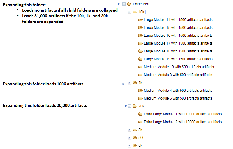 "FolderPerf" does not contain any artifacts, but it does contain 6 other folders (10k, 1k, 20k, 3k, 500, 5k). Those child folders in turn contain additional child folders which contain artifacts. If you expand "FolderPerf" for the first time, it will expand quickly and show you the 6 child folders. This operation is fast because the child folders don't contain any artifacts. Now, look at the 20k folder - this contains two child folders with 10,000 artifacts each. When expanding the 20k folder for the first time, 20,000 artifacts will be loaded into memory - and this can take a number of seconds. Second-time access to the folder will be fast, however (less than 1 second).
This is why a flat folder hierarchy can perform badly. If you put all of your folders under the root folder, then opening the folder will load all of the artifacts in your project area into memory. For a large project area, this could take several minutes, and is likely to result in a timeout.
Keep in mind that the user interface remembers which folders you have expanded. In the above example, the 1k, 20k, and 10k folders are expanded (for a total of 31,000 artifacts). If the DNG server is restarted, or if the artifacts are flushed out of memory, then opening the "FolderPerf" folder will load 31,000 artifacts into memory, which could be several minutes (or could result in a timeout).
There is also a relationship between modules and folders, since there is a folder for each module. If your project happens to include a "Modules" folder, expanding that folder can load all of the artifacts in all of the modules. That can take several minutes if you have 100,000 or more artifacts in modules.
If configuration management is enabled, you may pay the initial load penalty on folders or modules when switching between streams, or when creating a change set with the folder hierarchy visible. (This latter case was improved in the 6.0.5 release). You can avoid this penalty by making sure the folder hierarchy is not visible before you create a change set or switch streams.
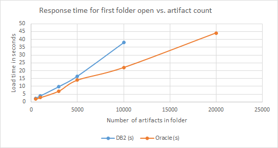
Here are response times (in seconds) for opening a folder for the first time, when no artifacts are cached. These are the worst cases; second time access should be less than 1 second. Note that on DB2, an attempt to open a folder with 20,000 artifacts timed out after 2 minutes, so there is no data point for that. Please refer to Appendix A for detailed test results involving folder loading.
"FolderPerf" does not contain any artifacts, but it does contain 6 other folders (10k, 1k, 20k, 3k, 500, 5k). Those child folders in turn contain additional child folders which contain artifacts. If you expand "FolderPerf" for the first time, it will expand quickly and show you the 6 child folders. This operation is fast because the child folders don't contain any artifacts. Now, look at the 20k folder - this contains two child folders with 10,000 artifacts each. When expanding the 20k folder for the first time, 20,000 artifacts will be loaded into memory - and this can take a number of seconds. Second-time access to the folder will be fast, however (less than 1 second).
This is why a flat folder hierarchy can perform badly. If you put all of your folders under the root folder, then opening the folder will load all of the artifacts in your project area into memory. For a large project area, this could take several minutes, and is likely to result in a timeout.
Keep in mind that the user interface remembers which folders you have expanded. In the above example, the 1k, 20k, and 10k folders are expanded (for a total of 31,000 artifacts). If the DNG server is restarted, or if the artifacts are flushed out of memory, then opening the "FolderPerf" folder will load 31,000 artifacts into memory, which could be several minutes (or could result in a timeout).
There is also a relationship between modules and folders, since there is a folder for each module. If your project happens to include a "Modules" folder, expanding that folder can load all of the artifacts in all of the modules. That can take several minutes if you have 100,000 or more artifacts in modules.
If configuration management is enabled, you may pay the initial load penalty on folders or modules when switching between streams, or when creating a change set with the folder hierarchy visible. (This latter case was improved in the 6.0.5 release). You can avoid this penalty by making sure the folder hierarchy is not visible before you create a change set or switch streams.
Here are response times (in seconds) for opening a folder for the first time, when no artifacts are cached. These are the worst cases; second time access should be less than 1 second. Note that on DB2, an attempt to open a folder with 20,000 artifacts timed out after 2 minutes, so there is no data point for that. Please refer to Appendix A for detailed test results involving folder loading.
 For the 6.0.3 release and later, you may be able to use components to reduce the first-time open penalty. If you can spread your artifacts across several small components (instead of having everything in one project area), you may be able to reduce the number of artifacts underneath any given folder.
That concludes my discussion of data organization and performance. Now, I'll move on to discuss how to keep track of how big your DNG repository is getting.
For the 6.0.3 release and later, you may be able to use components to reduce the first-time open penalty. If you can spread your artifacts across several small components (instead of having everything in one project area), you may be able to reduce the number of artifacts underneath any given folder.
That concludes my discussion of data organization and performance. Now, I'll move on to discuss how to keep track of how big your DNG repository is getting.
Monitoring the growth of a DNG repository
In this section, I'll look at the things you can monitor to see whether your DNG repository is nearing its limits. You can use this information to decide when to deploy a new DNG server, or whether you should improve the specs of your existing server.Monitoring artifact counts
There are several values related to artifact counts that are useful to monitor:- The total number of artifacts
- The total number of versions
- The number of artifacts per project area
- Number of configurations
- DB2: select count(*) from VVCMODEL.VERSION
- Oracle: select count(*) from rmuser.VVCMODEL_VERSION
- DB2: SELECT COUNT(*) FROM VVCMODEL.CONFIGURATION WHERE ARCHIVED = 0
- Oracle: SELECT COUNT(*) FROM rmuser.VVCMODEL_CONFIGURATION WHERE ARCHIVED = 0
PREFIX rm: <http://www.ibm.com/xmlns/rdm/rdf/>
PREFIX rdf: <http://www.w3.org/1999/02/22-rdf-syntax-ns#>
PREFIX dc: <http://purl.org/dc/terms/>
PREFIX jfs: <http://jazz.net/xmlns/foundation/1.0/>
PREFIX rrmNav: <http://com.ibm.rdm/navigation#>

SELECT ( count (distinct *) as ?count )
WHERE {
?Resource rdf:type rm:Artifact .
?Resource rrmNav:parent ?Parent
}
LIMIT 1
The second gives you the number of artifacts in each project area:
PREFIX dc: <http://purl.org/dc/terms/>
PREFIX rdf: <http://www.w3.org/1999/02/22-rdf-syntax-ns#>
PREFIX rdfs: <http://www.w3.org/2000/01/rdf-schema#>
PREFIX rm: <http://www.ibm.com/xmlns/rdm/rdf/>
PREFIX rmTypes: <http://www.ibm.com/xmlns/rdm/types/>
PREFIX rrmReview: <http://www.ibm.com/xmlns/rrm/reviews/1.0/>
PREFIX nav: <http://com.ibm.rdm/navigation#>
PREFIX jfs: <http://jazz.net/xmlns/foundation/1.0/>
PREFIX owl: <http://www.w3.org/2002/07/owl#>
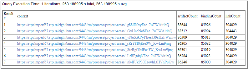
SELECT DISTINCT ?context ( count(?artifact) as ?artifactCount ) ( count(?binding) as ?bindingCount ) ( count (?link) as ?linkCount )
WHERE {
{?artifact rdf:type rm:Artifact .
OPTIONAL{?artifact rm:boundArtifact ?boundArt .}
FILTER (!BOUND(?boundArt)) .
?artifact jfs:resourceContext ?context
}
UNION
{?binding rdf:type rm:Artifact .
?binding rm:boundArtifact ?boundArt .
?binding jfs:resourceContext ?context
}
UNION {
?link rdf:type rm:Link .
?link jfs:resourceContext ?context
}
}
GROUP BY ?context
ORDER BY DESC (?artifactCount )
The output of the above query will be similar to the example shown below. You'll get a list of project areas, and the number of artifacts in each project area. You'll also get an idea of how many links you have, and how many "bindings", where there is a binding for each artifact that is in a module.
Monitoring the local index
You can also monitor the local DNG (Jena) index. Monitor how big it is by looking at the size of the rm/conf/indices directory (look specifically at the size of the jfs-rdfindex directory). Note that the location of the indices directory is configurable in rm/admin Advanced properties, so you may need to look at the Advanced Properties if your directory is not in the default location. On Linux, you can get an idea of the jfs-rdfindex size by using the "cd" command to move into the jfs-rdfindex directory, and then executing this command:du --block-size GYou can also get information about what's in the Jena index by executing a SPARQL query for "Resources and triples by artifact type". (See https://jazz.net/wiki/bin/view/Deployment/CalculatingYourRequirementsMetrics.) The query is:
PREFIX rdf: <http://www.w3.org/1999/02/22-rdf-syntax-ns#>
PREFIX rdfs: <http://www.w3.org/2000/01/rdf-schema#>
PREFIX rm: <http://www.ibm.com/xmlns/rdm/rdf/>
PREFIX rmTypes: <http://www.ibm.com/xmlns/rdm/types/>
PREFIX rrmReview: <http://www.ibm.com/xmlns/rrm/reviews/1.0/>
PREFIX nav: <http://com.ibm.rdm/navigation#>
PREFIX jfs: <http://jazz.net/xmlns/foundation/1.0/>
PREFIX owl: <http://www.w3.org/2002/07/owl#>

SELECT ?type (COUNT(*) AS ?no ) (COUNT(distinct ?resource ) AS ?graphs )
WHERE {
    ?resource rdf:type ?type .
    ?resource ?p ?o
} GROUP BY ?type
ORDER BY DESC(?no)
The output of this query will look something like this:
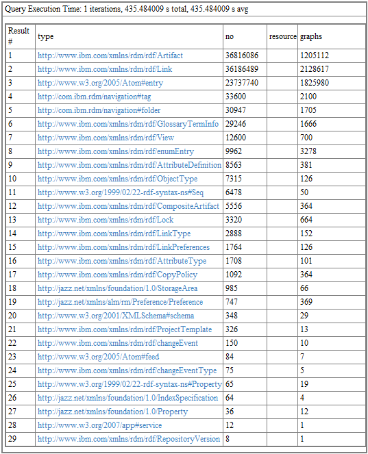 This may give you some insight into what people are doing with requirements. You can figure out what most of these entries represent from their type names; the Atom#entry type represents comments.
Monitoring the operating system
You can monitor statistics on usage of the page cache to determine whether you have enough RAM for your DNG workload. There are two things to look at:- How much of the local Jena index is loaded into the page cache (using linux-ftools)
- Paging rates (using pgpgin and pgpgout statistics available from sar or iostat)
Page cache occupancy
You can use a Linux utility called fincore (available in linux-ftools) to see how much of the Jena index has been loaded into the page cache. Jena uses memory-mapped files, and portions of these files will be brought into the page cache as they are accessed. If there is enough RAM available, the Jena index can be kept entirely in memory and this will improve performance. After downloading and compiling linux-ftools, you can run it against the files in the jfs-rdfindex directory (under server/conf/rm/indices/[root@test jfs-rdfindex]# linux-fincore --pages=false --summarize * filename size total_pages min_cached page cached_pages cached_size cached_perc -------- ---- ----------- --------------- ------------ ----------- ----------- GOSP.dat 6,954,156,032 1,697,792 -1 0 0 0.00 GOSP.idn 117,440,512 28,672 -1 0 0 0.00 GPOS.dat 6,937,378,816 1,693,696 -1 0 0 0.00 GPOS.idn 109,051,904 26,624 -1 0 0 0.00 GSPO.dat 6,928,990,208 1,691,648 0 1,024 4,194,304 0.06 GSPO.idn 109,051,904 26,624 0 2,048 8,388,608 7.69 index.properties 308 1 0 1 4,096 100.00 node2id.dat 587,202,560 143,360 0 140,450 575,283,200 97.97 node2id.idn 41,943,040 10,240 0 5,120 20,971,520 50.00 nodes.dat 1,405,294,013 343,090 0 343,052 1,405,140,992 99.99 OSP.dat 8,388,608 2,048 -1 0 0 0.00 OSPG.dat 6,207,569,920 1,515,520 -1 0 0 0.00 OSPG.idn 226,492,416 55,296 -1 0 0 0.00 OSP.idn 8,388,608 2,048 -1 0 0 0.00 POS.dat 8,388,608 2,048 -1 0 0 0.00 POSG.dat 6,274,678,784 1,531,904 3,598 1,521,482 6,231,990,272 99.32 POSG.idn 268,435,456 65,536 0 7,850 32,153,600 11.98 POS.idn 8,388,608 2,048 -1 0 0 0.00 prefix2id.dat 8,388,608 2,048 0 1,024 4,194,304 50.00 prefix2id.idn 8,388,608 2,048 0 1,024 4,194,304 50.00 prefixIdx.dat 8,388,608 2,048 -1 0 0 0.00 prefixIdx.idn 8,388,608 2,048 -1 0 0 0.00 SPO.dat 8,388,608 2,048 -1 0 0 0.00 SPOG.dat 6,215,958,528 1,517,568 3,588 1,513,686 6,200,057,856 99.74 SPOG.idn 109,051,904 26,624 0 24,522 100,442,112 92.10 SPO.idn 8,388,608 2,048 -1 0 0 0.00The cache_perc column tells you the percentage of the file contents that are currently resident in the page cache. For a large DNG repository, there will be a number of very large (multi-gigabyte) files with names like POSG.dat. You want to see high residency percentages for those files, since those are used in DNG queries. Lower residency numbers mean one of two things:
- There is not enough RAM to cache all of the files in the page cache.
- The pattern of access to DNG artifacts might not require all of the index. If you have a few active projects but many inactive projects, or if you have just restarted a server, you could see lower residency percentages.
Paging statistics
When DNG accesses Jena data that is not in memory, a page fault will be generated and part of the Jena index will be read into memory. The statistic pgpgin gives you information about the rate at which data is being brought in from disk due to page faults. The statistic pgpgout gives you information about the rate at which pages are written out of memory to disk. Pages become dirty when data is updated (like when you create or edit artifacts). Those pages will be flushed out to disk periodically. Note that Jena has a transaction feature similar to those seen in relational databases, so that queries or updates can operate on a consistent view of the data. When transactions are committed, even for queries that don't change data, Jena will force all dirty pages to be written out to disk. This overrides the default behavior of Linux with respect to dirty pages, so that changing Linux parameters like dirty_ratio will have little effect on DNG workloads. There are several different tools available for monitoring paging statistics. First, if you have enabled sar, you can get paging statistics via "sar -B". It is a good idea to enable sar, because it keeps historical data on system performance. This can be useful if you are having problems at a particular time of day - with sar, you can go back and see what was happening at that particular time. The output from "sar -B" is shown below, with the key columns being "pgpgin/s" and "pgpgout/s".[root]# sar -B Linux 3.10.0-514.10.2.el7.x86_64 (hostname) 01/24/2018 _x86_64_ (24 CPU) 12:00:01 AM pgpgin/s pgpgout/s fault/s majflt/s pgfree/s pgscank/s pgscand/s pgsteal/s %vmeff 12:10:01 AM 0.02 12.83 116.50 0.00 103.18 0.00 0.00 0.00 0.00 12:20:01 AM 0.00 7.39 132.41 0.00 160.37 0.00 0.00 0.00 0.00 12:30:01 AM 0.00 8.11 103.36 0.00 101.60 0.00 0.00 0.00 0.00You can monitor disk statistics using iostat. This tool looks at all disk I/O, not just paging statistics, so this can help you understand whether your disks are not able to handle the workload. "iostat -x" will give detailed statistics, as shown below. Trouble indicators can include high iowait percentages, high %util values for devices, and high read or write rates. The output below comes from a system which was having performance problems, so you can see some of those symptoms below. Sar will also give you disk i/o statistics (sar -d).
avg-cpu:  %user   %nice %system %iowait  %steal   %idle
          22.91    0.00    1.47   14.44    0.00   61.18

Device:         rrqm/s   wrqm/s     r/s     w/s    rkB/s    wkB/s avgrq-sz avgqu-sz   await r_await w_await  svctm  %util
sda               0.00    18.20 2444.60   10.80 204557.60   178.40   166.76    84.06   34.19   33.86  109.80   0.41  99.70
dm-0              0.00     0.00   90.00    4.00  2585.60    16.00    55.35     6.27   67.97   64.31  150.30   9.40  88.36
dm-1              0.00     0.00 2348.20   16.80 201885.60   123.20   170.83    79.88   33.68   33.08  117.32   0.42  99.10
dm-2              0.00     0.00    0.00    7.20     0.00    28.80     8.00     1.03  150.39    0.00  150.39  21.53  15.50
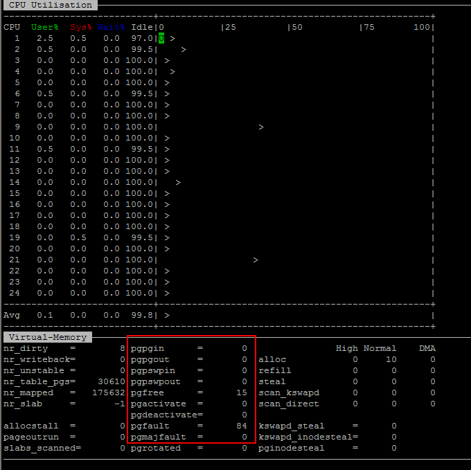
Another useful Linux utility is nmon. nmon can collect data periodically over time and turn it into an Excel spreadsheet, or it can be run in an interactive mode to let you see what's happening in real-time (see screenshot below). I will often keep nmon running in interactive mode during performance tests so I can spot signs of trouble. I'll usually display CPU utilization data, as well as virtual memory statistics (especially the paging stats). Also of interest is nr_mapped (number of pages mapped by files - e.g. Jena) and nr_dirty (number of dirty pages).
 You have probably been wondering whether are particular thresholds for all of these statistics that indicate problems. The good news is that those thresholds exist, but the bad news is that they will depend on your particular server hardware. There are a few things you can do:
 - Understand the maximum throughput for your disk drives, and compare that to the disk I/O rates from iostat or sar. You may want to benchmark the performance of your disks using a tool like sysbench.
- Collect baseline measurements during times of light, normal, and heavy load and use those measurements to estimate thresholds. If performance is good under light or normal load, then the measurements at those times are indicators of a healthy system. If you have periods of bad performance, then you can compare measurements from those times to the baseline in order to see which statistics are correlated with poor performance.
Final thoughts
This document is a deep-dive into factors that influence the performance of DOORS Next Generation, with a focus on the impact of repository size and data shape. I've covered:- The architectural factors with the most performance impact
- Ways of organizing DNG data and the limits of those features
- Ways of monitoring the size of a DNG repository
- Operating system metrics to monitor that can serve as warning signs of performance problems
- Test results for module and folder operations, covering DB2 and Oracle
- A case study looking at operating system metrics for a poorly-performing system
- Take advantage of the features available to organize your requirements, but stay under the recommended limits
- Make sure you have enough RAM to keep your Jena index in memory, and monitor your index size and add RAM over time as needed.
- Use the fastest possible disk drives available if you have large repositories
- Monitor your repository size and take action before you reach data limits
Appendix A - test results
Test methodology
The test approach was:- In rm/admin Advanced Properties, change the following properties:
- Set RDMRecentComments.query.modifiedsince.duration = 1
- Set RDMRecentRequirements.query.modifiedsince.duration = 1
- Set query.client.timeout to 240000
- Shut down the server, and restart it
- Open the dashboard for the test project, then select the artifacts menu
- Monitor rm/admin Active Services until the initialization queries complete
- Finally, execute the operation of interest manually, and measure the time to complete the operation using a stopwatch.
- If there are many recent changes or comments, the Linux page cache can be populated with DNG index data from Jena when opening the project dashboard. This can also add to the DNG server caches. My test project area did not have recent comments or changes (I lowered the recent comment/requirement duration setting to make sure I didn't pick up older changes).
- There are several caches within the database server, as well. SQL statements can be compiled and cached; data from database can be brought into memory as it is used.
Test topology
Servers
The test results discussed in this document were obtained from two different RM deployments, each of which used the same topology and hardware with one difference: one deployment used a DB2 database server, and the other used an Oracle database server. Any difference in response times will be due solely to the database. The tests used the 6.0.3 release (ifix8). WebSphere Liberty was used as the application server. The Jazz Authorization Server was used for authentication and single-signon.|
Function |
Number of machines |
Machine type |
Processor/machine |
Total processor cores/machines |
Memory/machine |
Network interface |
OS and version |
|
|
Proxy Server (IBM HTTP Server and WebSphere Plugin) |
1 |
IBM System x3250 M4 |
1 x Intel Xeon E3-1240v2 3.4 GHz (quad-core) |
8 |
16 GB |
Gigabit Ethernet |
Red Hat Enterprise Linux Server release 6.3 (Santiago) |
|
|
Jazz Team Server WebSphere Liberty |
1 |
IBM System x3550 M4 |
2 x Intel Xeon E5-2640 2.5 GHz (six-core) |
24 |
32 GB |
Gigabit Ethernet |
Red Hat Enterprise Linux Server release 7 |
|
|
RM server WebSphere Liberty |
1 |
IBM System x3550 M4 |
2 x Intel Xeon E5-2640 2.5 GHz (six-core) |
24 |
32G |
Gigabit Ethernet |
Red Hat Enterprise Linux Server release 7 |
|
|
Database server DB2 10.5 or Oracle 11.2.0.3 |
1 |
IBM System x3650 M4 |
2 x Intel Xeon E5-2640 2.5 GHz (six-core) |
24 |
64 GB |
Gigabit Ethernet |
Red Hat Enterprise Linux Server release 6.3 (Santiago) |
|
|
Network switches |
N/A |
Cisco 2960G-24TC-L |
N/A |
N/A |
|
Gigabit Ethernet |
24 Ethernet 10/100/1000 ports |
|
Data
The data shape used in these tests used 6 identical project areas, enabled for configuration management. The size of the Jena index on disk was 49G. Each project area included the following artifacts:|
Artifact type |
Number |
|
Large modules (10,000 artifacts) |
2 |
|
Medium modules (1500 artifacts) |
40 |
|
Small modules (500 artifacts) |
10 |
|
Folders |
119 |
|
Module artifacts |
85000 |
|
Non-module artifacts |
1181 |
|
Comments |
260582 |
|
Links |
304029 |
|
Collections |
14 |
|
Public tags |
300 |
|
Private tags |
50 |
|
Views |
200 |
|
Terms |
238 |
|
Streams |
15 |
|
Baselines |
15 |
|
Change sets |
600 |
Test results: opening modules and creating change sets
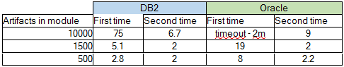
Here are test results for opening modules of various sizes, on a DB2 system and an Oracle system. In the following tests, I opened modules of varying sizes (500, 1500, and 10000 artifacts). I opened each module twice. Here are the times (in seconds) when opening modules from smallest to largest (first 500, then 1500, then 10000):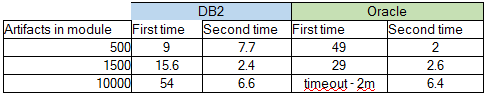 Here are the times when opening the modules from largest to smallest (first 10,000 then 1500 then 500):
 Here are times (in seconds) for creating change sets when viewing modules of various sizes. When a change set is created, the module contents are refreshed in the context of the new change set. Since the context is new, the module contents are not yet cached and need to be loaded.
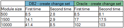 There is quite a bit of variation in the numbers, but there are some conclusions to be drawn:
 - Second time costs for module loading are in the 5-10 second range, and are not overly sensitive to module size. Once artifacts are cached, they are relatively fast to load.
- Modules of 10,000 artifacts can take a minute or more to load for the first time on DB2, and more than 2 minutes on Oracle. Timeouts occur at the 2 minute mark. This is what leads us to set the limit of artifacts per module at 10,000
- Because caching is not relevant during change set creation, the refresh times for larger modules can exceed 60 seconds if you create a change set while viewing the module.
- Oracle performs worse than DB2 for first-time module loading. The SQL statements executed during module loading are different for Oracle, and are more expensive to process.
- An analysis of SQL statements collected by repodebug during first time module open shows that roughly half of the time is spent in the database.
Test results: opening folders
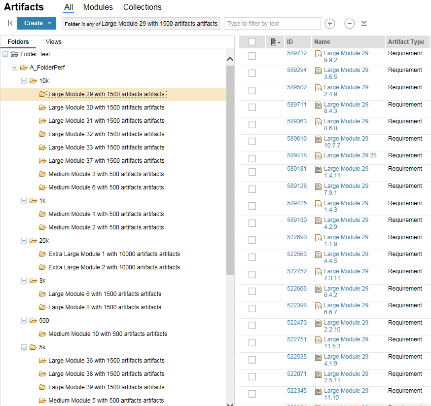
I created a folder hierarchy with a known set of artifacts in a test project area, and then measured the time it took to expand each folder, using a stopwatch. The test data was organized into a folder with 6 child folders.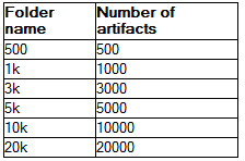 The child folders above contained folders for modules, so that expanding the child folders loaded the module folders and the artifacts in the module. The 3k folder, for example, included folders for 2 modules of 1500 artifacts each. The test folder hierarchy is shown below:
 The response times were not consistent, and in fact, varied depending on the order in which the folders were opened. The results were different if you opened the folders in order from smallest to largest than if you opened the folders from largest to smallest (at least on DB2). I attribute the difference to caching dynamics on the DB2 server (numbers on Oracle were more consistent). Despite the inconsistencies, we can still draw conclusions from the tests:
 - Most of the time is spent executing SQL statements
- Second-time opens are uniformly fast (less than 1s) and do not depend on the number of artifacts in the folder hierarchy.
- Open times increase linearly with the number of artifacts that need to be loaded from the database. The number of SQL calls issued is directly proportional to the number of artifacts in the folder hierarchy.
- As the number of artifacts to be loaded grows past 5000, you may need to increase the query.client.timeout beyond 30 seconds to avoid timeouts.
- DB2 performs worse than Oracle.
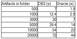 Here are the numbers when opening folders in order from largest to smallest:
 When opening from largest to smallest, the 20,000 artifact folder timed out on DB2, with this error:
 I used the querystats feature in rm/repodebug to look at where the time was going when opening a folder containing 10,000 artifacts on DB2. The breakdown below shows more than 80% of the time is spent in database operations (with most of that being SQL statements that are reading data). The "non-DB" time entry is the time spent in the DNG server doing things other than executing SQL queries.

Test results: monitoring the operating system
In this section, I'll look at what happens to various operating system metrics as a DNG server becomes overloaded. In this test, I used a server with 32G of RAM, and used a JVM heap size of 22G. This means that there is at most 10G of RAM available for the page cache. The local Jena index was 40G in size, so it could not all be cached in memory. The system used a regular hard drive (not an SSD). To prepare for the test, I stopped the DNG server and cleared the Linux page cache. Then, I restarted the DNG server. By starting the server this way, I ensured that the Jena index started out entirely on disk (no caching). Next, I applied a simulated 300 user workload to the system, and monitored it over time. Here is a summary of the results (with more details following later):- The performance of the system degraded sharply after 18 hours of run time.
- Over the course of the test, the amount of memory available to the page cache slowly decreased as the JVM used more memory. Although the JVM was configured with a 22G heap, it did not start out using the full 22G of RAM. The percentage of the Jena index cached in memory therefore went down over time (since the size of the page cache decreased).
- At the time the performance started to degrade, there were sharp increases in the following operating system metrics:
- Page ins per second
- Disk utilization
- Disk transfer rates
- Disk queue size
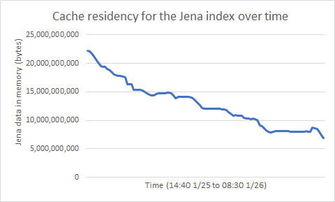
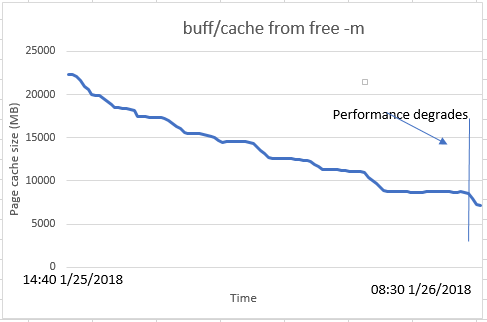 Using fincore, I looked at how much of the Jena index was resident in memory over the 18 hour test period (the Y axis below is in bytes). The previous graph shows the page cache shrinking, and as it does, there is less room for the Jena data and so there is less Jena data resident in memory over time. The fact that the residency percentage is going down is a red flag. When the page cache was larger early on, more of the Jena index was cached in memory and we can assume this was because the workload needed to access Jena data and therefore brought it into memory. If the residency numbers had stayed flat, we could assume there was enough memory to keep the needed Jena data in memory. But a downward trend in residency suggests that Jena data that was once needed has been paged out. That means that an alteration in the workload (like accessing a different project area) could suddenly result in a spike in disk activity as some data is brought back into memory (and other data is paged out).
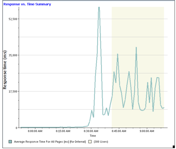
 Because the page cache is much smaller than the Jena index, the DNG server eventually must read Jena data into memory from disk, and this creates a bottleneck at the disk - the disk drive is not able to transfer data into memory at a high enough rate. Let's zoom in on the last hour of the test, when things go off the rails. First, let's look at the overall response times - performance starts to degrade around 8:15am, and then gets much worse around 8:30 (when the average overall response times are more than 50 seconds). The system is not responsive at this point.
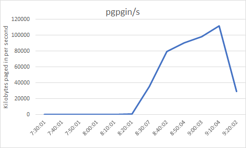
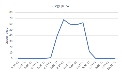
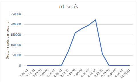
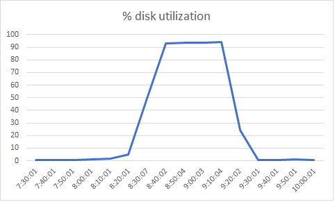
 The charts below are derived from sar output. The page-in rate (pgpgin/s) has sharply increased around the time performance degrades - since the page cache is much smaller than the Jena index, this shows that the Jena data is being read into memory from disk. But we can also see that the disk utilization has sharply increased and is near its maximum. So the speed of the disk has become a bottleneck - the server can't bring Jena data into memory fast enough, and this is causing DNG operations to slow down. The average queue size grows, which means that requests for I/O are having to wait for the disk to be available. Finally, we can see the number of 512 byte sectors (rd_sec/s) read from the device per second...this increases sharply as well, which is just a reflection of the high page-in rate. 150,000 sectors per second of 512 bytes each works out to around 75 megabytes per second, which is going to be pushing the limits for a hard drive (as the disk utilization numbers confirm).
References
Related topics:
- Sizing and tuning guide for Rational DOORS Next Generation 6.0.2: configuration management
- Sizing and tuning guide for Rational DOORS Next Generation 6.0: configuration management
- Tips for configuring and tuning DOORS Next Generation
- DNG View Query best practices
- Rational DOORS 9 to Rational DOORS Next Generation migration sizing guide
- Calculating your requirements metrics
External links:
- IBM
- Memory-mapped I/O - Wikipedia
- linux-ftools - tool for analyzing the Linux page cache
- nmon - Collect operating system metrics
- sysbench - OS benchmarking tool (includes disk I/O benchmarks)
- Garbage Collection and Memory Visualizer (GCMV)
Additional contributors: KnutRadloff


Contributions are governed by our Terms of Use. Please read the following disclaimer.
Dashboards and work items are no longer publicly available, so some links may be invalid. We now provide similar information through other means. Learn more here.