IBM Rational Software Architect Design Manager 4.0 Performance And Sizing Report
In this article we report the results of the performance and scalability testing we have done on Rational Software Architect Design Manager 4.0 (RSADM) and offer some guidance for planning its deployment and configuration. We executed automated multi-user tests to get performance data on a typical mix of use cases on a RSADM server under load. We also performed single-user tests of other important but less frequently used use cases. We performed performance tests on RSADM installed on dedicated hardware as well as on a virtual machine in a cloud environment hosted on an enterprise-class virtualization platform. The rest of this article describes this in more detail, presents our measurements and findings, and provides some guidance and advice for planning the deployment and configuration of RSADM.
Workload
To provide a reasonably realistic volume of model data for the tests, before each performance test run we imported into RSADM approximately 100 MB of model data comprising approximately 25,000 resources and over 800,000 total model elements. We performed two kinds of tests: multi-user tests of the most common use cases and single-user tests of other important, but less commonly used, operations.
During the development of RSADM we created an automated performance testing framework and test suite capable of simulating an arbitrary number of users executing a configurable mix of user-level operations (use cases) on a RSADM server over an arbitrary period of time. The framework drives the tests and records the response time of every user-level operation invoked during a test session. We used this framework and test suite to drive the multi-user tests and gather performance and response time data. The single-user tests were performed manually.
Multi-user tests
For the multi-user tests we used our performance test framework to simulate 1, 25 and 50 concurrent users performing a variety of common user operations over the course of approximately 1 hour. The use cases were split between the use of the two supported RSADM client types:
- Web client – A web browser
- Rich client – Rational Software Architect (RSA) with the Design Management (DM) extensions installed on it
The web client use cases were:
- Expand a explorer tree node – Simulates a user expanding a node in the Explorer tree.
- Create a resource – Creates an Ontology using forms.
- save a resource – Changes the title of an Ontology and saves it.
- Lock a resource – Locks an Ontology (implies the intent to modify it).
- Unlock a resource – Unlocks an Ontology that was previously locked.
- Open a resource – Simulates opening a resource in a form-based editor.
- Open a diagram – Simulates opening a UML diagram.
- Add a comment – Creates a textual comment on a resource.
- Search for resources – Searches for a keyword in all models in all project areas, retrieving additional information about the matching resources.
- Search for diagrams – Same as above except that it searches in diagrams only.
- Get a OSLC representation – Simulates a client requesting the OSLC representation of a resource.
The rich client uses cases were:
- Expand a explorer tree node – Simulates a user expanding a node in the Explorer tree.
- Open properties for a UML resource – Simulates showing a model element’s properties in the Properties Viewer.
Note that in most cases each test case execution issues more than one, sometimes several, server requests in order to emulate the requests that a web client or rich client would make for a particular use case. For example, the ‘Open a resource’ test, in addition to retrieving the form-based representation of the resource, also retrieves any existing comments, retrieves the ‘breadcrumbs’ (hierarchical path), etc.
For the multi-user tests, we aimed for a mix of 70% read operations and 30% write operations. Table 1 shows, for each use case, the number of simulated users and execution frequencies we used for the 25 and 50 user tests.
| Client type | Use case | 25 users | 50 users | Notes | ||||
|---|---|---|---|---|---|---|---|---|
| Number of users | Execution rate (per minute) | Number of users | Execution rate (per minute) | |||||
| Per-user | Net | Per-user | Net | |||||
| Web client | Expand a explorer tree node | 2 | 1 | 2 | 4 | 1 | 4 | |
| Create a resource | 2 | 8/9 | 1⅞ | 5 | ¾ | 3¾ | ||
| Save a resource | 3 | ⅚ | 2½ | 5 | 1 | 5 | ||
| Lock a resource Unlock a resource | 2 | 1¼ 1¼ | 2½ 2½ | 5 | 1 1 | 5 5 | Each simulated user executes both use cases. | |
| Open a resource | 2 | ⅝ | 1¼ | 5 | ½ | 2½ | ||
| Open a diagram | 2 | ⅝ | 1¼ | 5 | ½ | 2½ | ||
| Add a comment | 3 | ⅚ | 2½ | 5 | 1 | 5 | ||
| Search for resources | 2 | ¾ | 1½ | 3 | 1 | 3 | ||
| Search for diagrams | 1 | 1 | 1 | 2 | 1 | 2 | ||
| Get OSLC representation | 3 | ⅚ | 2½ | 5 | 1 | 5 | ||
| Rich client | Expand a explorer tree node | 2 | 1 | 2 | 4 | 1 | 4 | |
| Open properties for a UML resource | 1 | 1 | 1 | 2 | 1 | 2 | ||
| Total: | 25 | 24⅜ | 50 | 48¾ | ||||
This distribution resulted in 28.2% of the total net operations being write operations (“Create a resource”, “Save a resource” and “Add a comment”), which is quite close to the 30% we were aiming for.
Single-user tests
The single-user tests are what are expected to be relatively lower-frequency (but still important). The use cases were:
- Finalize RSADM setup – Finalize the RSADM application during server setup on Tomcat using the default Derby database configuration.
- Import 100 MB model data
- Re-import 100 MB model data – Re-import the 100 MB of model data in which approximately 6% of its resources have been modified.
- Create a workspace (from a snapshot)
- Create a snapshot
- Run a report – Run a report on a model using the UML metrics report template supplied with Design Manager.
- Run an impact analysis – Run an impact analysis on a UML component using 3 levels of depth and the default configuration and views.
Test environments
Hardware configurations
We tested RSADM in two environments, one on a virtual machine hosted on an enterprise-class virtualization platform and the other on a dedicated server.
The virtual machine on which we tested RSADM was hosted on an enterprise-class virtualization platform consisting of a cluster of 7 IBM System x3850 X5 servers each with 4 8-core x 2-thread 64-bit Intel® Xeon® X7550 CPUs running at 2 GHz (224 CPU cores total) with a total of 4.25 TB of RAM. This was connected to an IBM System Storage DS8800 with a capacity of 100 TB. See Figure 1. The server cluster was lightly loaded, typically running at approximately 20% of capacity.
Figure 1: Virtual machine host platform hardware configuration 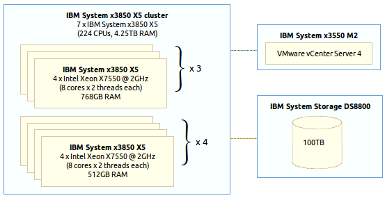
The virtual machine was configured with 2 CPUs (2 cores total), 8 GB RAM, and 100 GB of disk storage running under the VMWare® ESX 4.1.0 hypervisor. See Figure 2.
Figure 2: Virtual machine hardware configuration 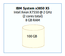
The dedicated server on which we tested RSADM was an IBM System x3850 X5 server with 4 6-core 64-bit Intel Xeon X7542 CPUs running at 2.67 GHz (24 CPU cores total) with 128 GB of RAM and 1 TB of local disk storage. See Figure 3.
Figure 3: Dedicated server hardware configuration 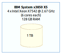
Software configurations
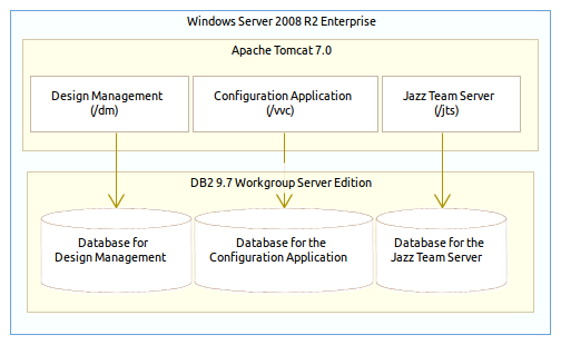
In order to effectively plan for the deployment of RSADM it is important to have at least a high-level understanding of its major components and their interactions. Figure 4 illustrates these components and interactions, also showing the different types of clients.
Figure 4: Component relationships and interactions in RSADM 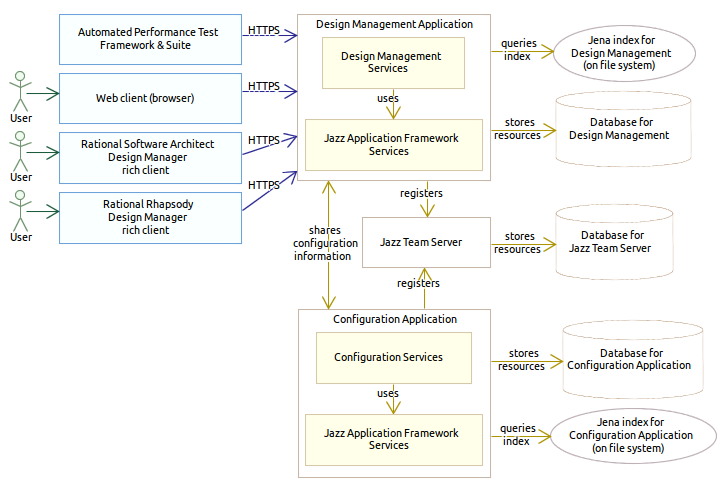
There are three general types of components, loosely arranged in Figure 4 into three columns:
- On the left are the various client types supported.
- In the center column are the web applications that comprise a minimal RSADM installation. Each of these is a distinct web application which could be run on the same application server or on separate ones (which may be run on separate machines).
- The Design Management Application provides Design Management services to clients via HTTP/HTTPS.
- The Configuration Application stores and manages configuration and version metadata of resources for Jazz applications (RSADM in this case).
- The Jazz Team Server provides common services for Jazz applications (e.g., user management and authentication).
- On the right are the data stores used by the applications.
- Each application has a database which it uses to store its application-specific data. Depending on scalability needs and the database implementation being used, each database may be local or accessed remotely.
- The Design Management and Configuration applications each maintain indices for quickly searching for information about the resources they store and manage. The index is a Jena-based Resource Description Framework (RDF) triplestore which resides on the application’s local file system. See the Storage requirements section for more details.
The deployment and configuration of RSADM were almost the same on both machines. Figure 5 shows this graphically:
- The operating system was Microsoft Windows Server 2008 R2 Enterprise (64-bit).
- We used IBM DB2® 9.7 Workgroup Server Edition for the databases.
- We ran the RSADM applications (Design Management and Configuration applications) and the Jazz Team Server (JTS) on a single instance of Apache Tomcat 7.0 (the version that ships with RSADM)
- We ran Tomcat on the IBM Java™ SE Runtime Environment 1.6.0 that is installed with RSADM.
- We used the Tomcat user registry to store user information.
There were a couple of differences in the configuration of RSADM between the virtual machine and the dedicated server. On the virtual machine, we ran RSADM with the default JVM settings as set in the server-startup script. On the dedicated server, in order to take advantage of its large amount of RAM, we changed -Xms and -Xmx to 50G (default is 4G) and -Xmn to 25G (default is 512M). On the dedicated server we also removed the -Xcompressedrefs and -Xgc:preferredHeapBase=0x100000000 arguments (which are present by default).
The multi-user tests were driven by our automated performance test framework and suite running on a separate virtual machine hosted on the same virtualization platform that hosted the RSADM virtual machine.
Results
Multi-user test results
Table 2 summarizes the mean response times that we recorded running the 25-user and 50-user tests on RSADM for 1 hour each on the virtual machine and on the dedicated server. All times are shown in seconds ± one standard deviation (σ). As before, the “Web client” client type refers to a web browser, while “Rich client” refers to Rational Software Architect (RSA) with the Design Management (DM) extensions installed on it.
| Client type | Use case | Mean response time (seconds ± σ) | |||
|---|---|---|---|---|---|
| 25 users | 50 users | ||||
| Virtual machine | Dedicated server | Virtual machine | Dedicated server | ||
| Web client | Expand a explorer tree node | 1.24 ± 0.34 | 1.22 ± 0.36 | 1.95 ± 1.37 | 1.25 ± 0.26 |
| Create a resource | 4.15 ± 1.50 | 4.41 ± 1.63 | 6.38 ± 2.65 | 4.71 ± 1.31 | |
| Save a resource | 3.80 ± 1.18 | 3.87 ± 1.08 | 5.86 ± 2.39 | 4.50 ± 1.31 | |
| Lock a resource | 0.33 ± 0.94 | 0.36 ± 0.61 | 0.99 ± 2.12 | 0.76 ± 1.05 | |
| Unlock a resource | 1.09 ± 0.67 | 1.14 ± 0.89 | 1.16 ± 0.84 | 1.21 ± 0.72 | |
| Open a resource | 6.56 ± 3.64 | 6.27 ± 3.50 | 7.10 ± 2.99 | 5.44 ± 1.63 | |
| Open a diagram | 0.71 ± 0.44 | 0.67 ± 0.53 | 1.55 ± 2.07 | 0.83 ± 0.63 | |
| Add a comment | 0.75 ± 1.08 | 0.66 ± 0.90 | 0.82 ± 0.93 | 0.72 ± 0.81 | |
| Search for resources | 0.46 ± 0.16 | 0.49 ± 0.22 | 0.80 ± 0.71 | 0.50 ± 0.21 | |
| Search for diagrams | 2.06 ± 1.72 | 1.76 ± 1.34 | 3.54 ± 3.37 | 1.88 ± 1.46 | |
| Get OSLC representation | 0.44 ± 0.94 | 0.49 ± 0.94 | 0.96 ± 1.64 | 0.67 ± 0.87 | |
| Rich client | Expand a explorer tree node | 3.12 ± 0.45 | 3.13 ± 0.60 | 4.23 ± 1.17 | 3.43 ± 0.45 |
| Open properties for a UML resource | 0.43 ± 0.95 | 0.22 ± 0.34 | 0.56 ± 0.95 | 0.45 ± 0.67 | |
Figure 6 shows these results graphically, making it easier to compare the times from the tests run on the virtual machine to those run on the dedicated server. Each short horizontal bar indicates the mean response time for that use case (in seconds). Each vertical bar indicates the range of ±1 standard deviation from that mean. For almost every use case, the mean response time on the dedicated server is a bit less than it is on the virtual machine. The standard deviations (variability) are smaller as well.
Figure 6: Response times from 25 and 50 user performance tests 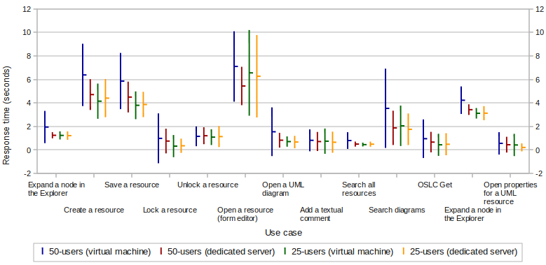
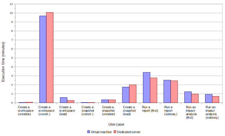
Single-user test results
Table 3 summarizes the execution times that we recorded from running the single-user tests of the low-frequency use cases on the virtual machine and dedicated server. Times are shown in hours, minutes and seconds. For the “Create a workspace” and “Create a snapshot” use cases, three times are reported:
- Creation – After clicking the “Create” button, the amount of time until the “Create successful” message appears.
- Construction – After creation, the amount of time that the workspace or snapshot remains “under construction” before it can actually be used.
- Load – After construction, the amount of time it takes to load the new workspace or snapshot (i.e., in the Explorer).
For the “Run a report” and “Run an impact analysis” use cases, two times are reported:
- First run – The amount of time it takes for the first run of a report or impact analysis to complete.
- Subsequent runs – The mean time it takes for subsequent runs of a report or impact analysis to complete.
| Use case | Time (hh:mm:ss) | ||
|---|---|---|---|
| Virtual machine | Dedicated server | ||
| Finalize Design Manager setup | 10:13 | 10:36 | |
| Import 100 MB model data | 1:38:00 | 1:45:00 | |
| Re-import 100 MB model data | 38:26 | 36:18 | |
| Create a workspace | Creation | 0:01 | 0:03 |
| Construction | 9:40 | 10:04 | |
| Load | 0:35 | 0:15 | |
| Create a snapshot | Creation | 0:01 | 0:01 |
| Construction | 0:20 | 0:19 | |
| Load | 1:45 | 1:59 | |
| Run a report | First run | 3:22 | 2:45 |
| Subsequent runs | 2:30 | 2:26 | |
| Run an impact analysis | First run | 1:13 | 0:57 |
| Subsequent runs | 0:55 | 0:43 | |
Figures 7 and 8 show these results graphically.
Figure 7: Execution times from the “Finalize Design Manager setup”, “Import 100 MB model data”, and “Re-import 100 MB model data” use case tests 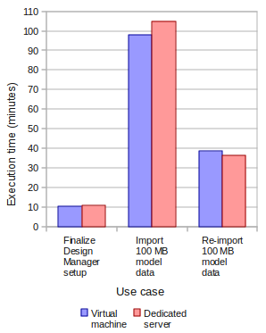
Import time details
In order to get a better understanding of the relationship between import time and the size of the model data being imported, we timed the import of several workspaces containing different amounts of model data. We did this only on the virtual machine because we saw little difference in import times between it and the dedicated server. Table 4 and Figure 9 summarize our findings.
| Model | Size of imported model data (MB) | Import time (minutes) | Import rate (minutes/MB) |
|---|---|---|---|
| JKE Banking Sample | 0.4 | 1.5 | 4.3 |
| A | 2.2 | 3.8 | 1.7 |
| B | 22.2 | 26.0 | 1.2 |
| C | 39.5 | 77.0 | 1.9 |
| D | 46.1 | 90.0 | 2.0 |
| E | 101.0 | 108.0 | 1.1 |
| Totals: | 211.4 | 306.3 |
For all but trivially small imports (i.e., if we consider models A-E only) this works out to very roughly 1.4 ± 0.4 minutes / MB of imported model data.
Figure 9: Size of imported model data vs. import time 
Server resource utilization
In addition to the 1-hour multi-user and single-user tests reported above, we ran the 50-user tests continuously for 5 days (on the virtual machine only) and periodically collected resource utilization data from the JVM running the RSADM server. We also installed and enabled some additional server instrumentation code on the server to enable us to collect additional application-specific information (such as statistics on the number of open HTTP connections). We recorded the following:
- Heap memory usage – The amount of memory being used for the Java heap as reported by the JVM.
- CPU utilization – The fraction of available CPU cycles being used as reported by the JVM (Note that the maximum is 200% rather than 100% because the virtual machine was configured with 2 CPU cores).
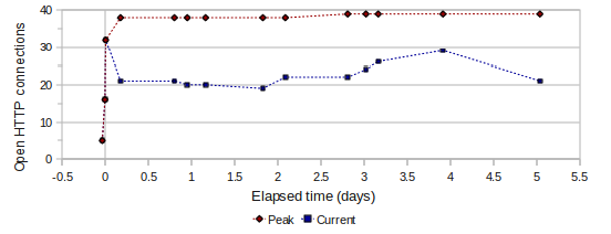
- Number of open HTTP connections – The number of open connections being used for HTTP requests as by our instrumentation code.
Table 5 summarizes the results. For each measurement, the maximum is the largest measurement we recorded, while the peak is continuously monitored by the JVM (for heap memory usage and CPU utilization) or our server instrumentation code (for open HTTP connections). The peaks exceed the maximums because none of our recorded measurements happened to be taken a point in time when any current value was at its peak.
| Measurement | Mean | Minimum | Maximum | Peak |
|---|---|---|---|---|
| Heap memory usage (GB) | 3.0 ± 0.65 | 1.6 | 3.7 | 4.0 |
| CPU utilization | 51% ± 31% | 0% | 98% | 201% |
| Number of open HTTP connections | 23.1 ± 4.0 | 19 | 32 | 39 |
Figures 10-12 graphically show the data collected over the 5-day run, including both current and peak measurements.
Figure 10: Heap memory usage during 5-day, 50-user test 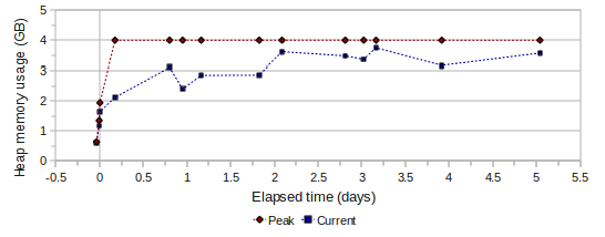

Storage requirements
Using the same set of models as we did in the ‘Import time details’ section, we also measured the storage space used by the imported model data. For a Jazz-based application such as RSADM, there are two significant types of storage: the databases and the indices.
The databases are where each Jazz application stores its application-specific data. In our setup (which would be typical for RSADM installed by itself) there were three, one each for RSADM, the Configuration Application and the JTS, all accessed locally. After database creation, server setup (which creates the database tables), and each import we recorded the total local disk space used by the databases as well as the size of each database (as reported by the DB2 Control Center).
The indices are Jena RDF triplestores in which each Jazz application stores metadata about the resources it manages in order to be able to support quickly searching and locating them. The indices reside on the local file system under <install>/server/conf/<application>/indices where <install> is the directory in which RSADM is installed (e.g., C:Program FilesIBMJazzTeamServer on Windows) and <application> is the per-application directory (“dm” for RSADM, “vvc” for the Configuration Application, and “jts” for the JTS). So, for example, in a default installation on Windows these would be:
- C:Program FilesIBMJazzTeamServerserverconfdmindices
- C:Program FilesIBMJazzTeamServerserverconfvvcindices
- C:Program FilesIBMJazzTeamServerserverconfjtsindices
After server setup and after each import we recorded the total disk space used in each of these directory trees. (Note that initially, just after installation, there are no indices.)
Databases
Table 6 shows the cumulative and incremental sizes of the databases after each import. Figure 13 shows the incremental database growth graphically.
| Model | Size of imported model data (MB) | Size of databases (cumulative GB) | Size of databases (incremental GB) | ||||||
|---|---|---|---|---|---|---|---|---|---|
| DM | VVC | JTS | Total | DM | VVC | JTS | Total | ||
| post-install | 0.100 | 0.100 | 0.100 | 0.299 | 0.100 | 0.100 | 0.100 | 0.299 | |
| post-setup | 0.632 | 0.600 | 0.568 | 1.800 | 0.532 | 0.500 | 0.469 | 1.501 | |
| JKE | 0.4 | 0.639 | 0.602 | 0.568 | 1.809 | 0.007 | 0.002 | 0.000 | 0.009 |
| A | 2.2 | 0.716 | 0.611 | 0.568 | 1.896 | 0.077 | 0.010 | 0.000 | 0.087 |
| B | 22.2 | 1.009 | 0.705 | 0.568 | 2.282 | 0.293 | 0.094 | 0.000 | 0.387 |
| C | 39.5 | 1.816 | 0.974 | 0.572 | 3.362 | 0.808 | 0.269 | 0.004 | 1.080 |
| D | 46.1 | 2.758 | 1.282 | 0.572 | 4.612 | 0.941 | 0.309 | 0.000 | 1.250 |
| E | 101.0 | 3.878 | 1.627 | 0.572 | 6.077 | 1.120 | 0.345 | 0.000 | 1.465 |
| Totals: | 211.4 | 3.878 | 1.627 | 0.572 | 6.077 | ||||
For each MB of imported model data we saw database size growth of roughly 20.7 MB, but there was a fair amount of variability (ranging from about 15 MB to 40 MB).
Figure 13: Size of imported model data vs. increase in size of databases 
Indices
Table 7 shows the cumulative and incremental sizes of indices and number of triples in the indices after each import. Figures 14 and 15 graphically show the index size growth and triples increase, respectively.
| Model | Size of imported model data (MB) | Size of indices (cumulative GB) | Size of indices (incremental GB) | Number of triples in indices (cumulative millions) | Number of triples in indices (incremental millions) | ||||||||||||
|---|---|---|---|---|---|---|---|---|---|---|---|---|---|---|---|---|---|
| DM | VVC | JTS | Total | DM | VVC | JTS | Total | DM | VVC | JTS | Total | DM | VVC | JTS | Total | ||
| post-install | 0.000 | 0.000 | 0.000 | 0.000 | 0.000 | 0.000 | 0.000 | 0.000 | 0.0 | 0.0 | 0.0 | 0.0 | 0.0 | 0.0 | 0.0 | 0.0 | |
| post-setup | 0.334 | 0.022 | 0.000 | 0.357 | 0.334 | 0.022 | 0.000 | 0.357 | 0.9 | 0.0 | 0.0 | 1.0 | 0.9 | 0.0 | 0.0 | 1.0 | |
| JKE | 0.4 | 0.346 | 0.024 | 0.000 | 0.371 | 0.012 | 0.002 | 0.000 | 0.014 | 1.0 | 0.0 | 0.0 | 1.0 | 0.0 | 0.0 | 0.0 | 0.0 |
| A | 2.2 | 0.406 | 0.030 | 0.000 | 0.436 | 0.060 | 0.006 | 0.000 | 0.065 | 1.1 | 0.1 | 0.0 | 1.2 | 0.2 | 0.0 | 0.0 | 0.2 |
| B | 22.2 | 0.999 | 0.078 | 0.000 | 1.078 | 0.593 | 0.048 | 0.000 | 0.642 | 3.0 | 0.2 | 0.0 | 3.1 | 1.8 | 0.1 | 0.0 | 1.9 |
| C | 39.5 | 2.178 | 0.218 | 0.000 | 2.396 | 1.179 | 0.139 | 0.000 | 1.318 | 6.5 | 0.5 | 0.0 | 7.0 | 3.6 | 0.3 | 0.0 | 3.9 |
| D | 46.1 | 3.493 | 0.381 | 0.000 | 3.874 | 1.315 | 0.164 | 0.000 | 1.478 | 10.5 | 0.8 | 0.0 | 11.3 | 3.9 | 0.3 | 0.0 | 4.3 |
| E | 101.0 | 5.913 | 0.581 | 0.000 | 6.494 | 2.420 | 0.200 | 0.000 | 2.620 | 18.3 | 1.2 | 0.0 | 19.5 | 7.8 | 0.4 | 0.0 | 8.2 |
| Totals: | 211.4 | 5.913 | 0.581 | 0.000 | 6.494 | 1.2 | 0.0 | 19.5 | |||||||||
For each MB of imported model data we saw index size growth of roughly 29.7 MB, ranging from about 27 MB to 40 MB, but the variability was much less than the variability of the database size growth, and the relationship is much closer to linear. Also, for each MB of imported model data we saw the number of triples in the indices increase by roughly 92,000, ranging from about 81,000 to 106,000. Again, the variability was much less than the variability of the database growth and the relationship is much closer to linear.
Figure 14: Size of imported model data vs. increase in index size 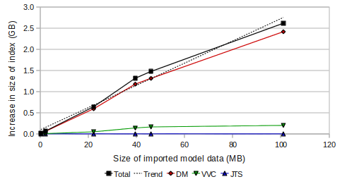

Hardware sizing recommendations
We showed that RSADM can support at least 50 users on the virtual machine and dedicated server environments we tested on using Tomcat, DB2, and a local Tomcat user registry (i.e., we did not use LDAP). Depending on your particular user load, you may be able to scale this down or you may need to scale it up. Table 8 summarizes how the virtual machine and dedicated server we used compare with the what is documented in the Rational Software Architect Design Manager system requirements. As you can see, our virtual machine met the requirements, but just barely, while the dedicated server far exceeded them. The performance numbers seem to reflect this. We probably would not want to try to support more than 50 users on this virtual machine configuration.
| Virtual Machine | Dedicated Server | RSADM Hardware Requirements | |
|---|---|---|---|
| CPUs | 2 cores | 24 cores (4 CPUs with 6 cores each) | 2 to 4 cores |
| RAM | 8 GB | 128 GB | 4 GB, 8+ GB recommended |
| Architecture | 64-bit | 64-bit | 64-bit (32-bit supported only for small-scale evaluation or demonstration purposes) |
Application server configurations
Our test environment configuration corresponds most closely to the “Departmental topology” described in the RSADM documentation section “Choosing an installation topology“. We ran the Design Management and Configuration applications and the JTS on a single server and on the same instance of the Tomcat application server. While this was sufficient for our 50-user test load to perform reasonably, for a larger-scale deployment we would recommend using WebSphere Application Server (WAS) and a distributed topology. Besides its scalability advantages, support for clustering, high availability, etc., WAS has several other features that make it particularly well-suited for hosting RSADM and other Jazz-based Collaborative Lifecycle Management (CLM) applications, including better support for single sign-on (SSO) and reverse proxy. See the Collaborative Lifecycle Management 2012 Sizing Report for a few more details. In general, the recommendations outlined there are applicable to RSADM as well, especially if you are integrating RSADM with CLM Applications.
Network connectivity
In our test configurations we ran the Design Management, Configuration and JTS applications using a local DB2 database. It can be a good load balancing strategy to move one or more of the databases to other machines and have the server access them remotely. In this case, however, network connectivity (especially latency) between the Jazz application server(s) and the database server(s) becomes a key factor. The Collaborative Lifecycle Management 2012 Sizing Report recommends no more than 1-2 ms latency and to locate the servers on the same subnet. This would apply to a RSADM deployment as well.
You could also choose to run the JTS on a different server than RSADM. This would typically be the case in a large RSADM deployment, especially if integrated with CLM applications. You might deploy the Design Management, Configuration and JTS applications each on a different server. In this case, good network connectivity between each application server and the JTS is important.
Artifact sizing guidelines
- Repository database
- If you use one of the supported DB2 or Oracle® database applications there are no hard limits to the number of project areas or users you can host. There is a limit of 10 registered users if you are using Apache Derby.
- Concurrent users
- Unless you are using Apache Derby for the repository database there is no hard limit on the number of users RSADM will support (other than what is effectively imposed by your hardware and deployment topology). Our performance testing has demonstrated that RSADM will support up to 50 concurrent users with reasonable response times on the configurations we tested. With more users than this we would expect to see higher response times.
- Model import
- There is no hard upper limit to the size of a model project being imported. The model data we imported for the performance tests reported here was approximately 100 MB in size comprising approximately 25,000 resources and over 800,000 total model elements.
Importing can impact server performance, so if you have large amounts of model data that needs to be imported we recommend using an automated import process scheduled for when there are few active users (e.g., outside of business hours). You should also consider limiting imports to one at a time.
Performance tuning
The performance tuning considerations for RSADM are similar to those for other Jazz-based applications (see, for example, the Rational Requirements Composer (RRC) 4.0 performance and tuning guide).
- Comply with the Hardware sizing recommendations: 64-bit architecture, 2-4 CPU cores, and at least 8 GB RAM.
- Configure the number of available TCP/IP ports to be the maximum supported by the host operating system and hardware. See below for instructions.
- Increase the size of the thread pool used by the server’s web application container from the default. See below for recommendations and instructions.
- Set the size of the heap the JVM uses appropriately. See below for recommendations and instructions.
Number of available TCP/IP ports
On AIX and Linux the default number of TCP/IP ports available is too low. To increase it, issue the following command:
ulimit -n 65000
On Windows the default number of available TCP/IP ports is higher than on AIX or Linux, but should still be increased.
- Windows Server 2008
-
See the instructions at http://support.microsoft.com/kb/929851. Set the start port to 2000 and the number of ports to 63535.
- Windows Server 2003
-
Open the registry. Under
HKEY_LOCAL_MACHINE/SYSTEM/CurrentControlSet/Services/Tcpip/Parameters, create a new DWORD named “MaxUserPort” and set its value to 65000. Reboot the machine for the change take effect.Note: Be very careful when modifying the Windows registry. Incorrect changes to the registry have the potential to cause Windows to behave erratically or to become inoperable. Always backup the registry before modifying it.
Thread pool size
The size of the thread pool used by the RSADM server’s web application container should be at least 2.5 times the expected active user load. For example, if you expect to have 100 concurrently active users, set the thread pool size to at least 250.
For Tomcat 7, refer to the “Executor (thread pool)” section in the Apache Tomcat 7 documentation.
For WebSphere Application Server (WAS), open the administrative console and select Servers ⇒ Server Types ⇒ WebSphere application servers ⇒ server name ⇒ Thread pools. See the “Thread pool settings” section in the WAS information center for more details.
JVM heap size
The maximum JVM heap size should be set to 4 GB if the server has at least 6 GB of RAM. If the server only has 4 GB RAM (not recommended) you may want to experiment with configuring a maximum JVM heap size of 2 GB or 3 GB. However, avoid setting the maximum JVM heap size to more than about 70-80% of the amount of RAM the server has or you may experience poor performance due to thrashing.
If you are running Tomcat, edit the server-startup script and change the values of -Xms and -Xmx to the desired values. You will need to stop and restart the server for the changes to take effect.
If you are running WAS, see the “Java virtual machine settings” section in the WAS information center for instructions specific to your WAS deployment.
For more information
On jazz.net:
- Check out Rational Software Architect Design Manager & Rational Rhapsody Design Manager.
- Download an evaluation version of Rational Software Architect Design Manager.
- From the jazz.net Library:
- The Collaborative Lifecycle Management 2012 Sizing Report (Standard Topology E1) describes the results of performance tests of the CLM 4.0 release and gives sizing and deployment topology recommendations for it.
- The Rational Requirements Composer 4.0 performance and tuning guide provides the results of performance and scalability tests of RRC 4.0 and offers some recommendations for configuring it.
- In Keeping my Jazz Server happy and my users overjoyed you will find some useful guidelines on maintaining the health of your Jazz application deployments.
Product documentation and support:
- On-line help (product documentation) – See especially the section on “Installing and configuring Rational Software Architect Design Manager 4.0“.
- For system requirements, see Rational Software Architect Design Manager System requirements for a summary. For more details go to Detailed system requirements for a specific product. Enter “Design Manager” as the product name and click “Search”. Select “Rational Software Architect Design Manager” in the search results, select version 4.0, select an operating system family, and click “Submit”.
- Support portal for Rational Software Architect
- Support portal for Rational Rhapsody family
- Collaborative Lifecycle Management 4.0 information center
Acknowledgements
The authors wish to express sincere appreciation to the following members from the performance team for their contributions to the performance framework and to many sections in this article related to measurements and findings.
- Nicholas Bennett, Senior Software Developer, IBM Rational
- Adam Mooz, Software Developer, IBM Rational
- Alex Fitzpatrick, Software Developer, IBM Rational
- Wayne Diu, Software Developer, IBM Rational
- Gleb Sturov, Software Developer, IBM Rational
- Alex Hudici, Student, IBM Rational
Summary and Next Steps
Rational Software Architect’s Design Management capability integrates architecture and design into Rational’s Solution for Collaborative Lifecycle Management.
Design Management provides many features including: a central design repository, Web client access to designs, change control and configuration management for designs, lifecycle traceability, dashboards, searching, impact analysis, document generation, commenting and markup of designs and design reviews.
The Design Management project on jazz.net offers a 60 day trial so you can download and try it out. The trial includes design artifacts for a sample application call Money That Matters that makes it easy to try out the features covered in this article. Additionally the library section on jazz.net contains articles, videos and other resources you may find helpful in learning more.
Copyright © 2012 IBM Corporation