Deep Dive Data Warehouse Reporting using the Jazz Reporting Service

Dr. Einar W. Karlsen
IBM Deutschland GmbH
Last updated: March 2015
Build basis: CLM 5.0.2

Summary

The Jazz Reporting Service is the new reporting solution from IBM Rational Software developed on top of the Jazz integration platform and is intended to support the authoring of custom reports for the Collaborative Lifecycle Management (CLM) solution. A previous articles around Jazz Reporting Service covered reporting using the build in query builder [Haumer 2014], which allows end users to create their own reports almost right away with simple drag-and-drop gestures and selections. Another article [Shaw 2014] went one step further and demonstrated how to use the Structured Query Language (SQL) editor to modify and refine the underlying SQL statement that were generated by the query builder introducing some more advanced features.

In this article I will take the excursion into Jazz Reporting Service one step further in two ways. First of all you will see how Jazz Reporting Service can be used to report on data in the Data Warehouse that is not exposed by the query builder simply by by-passing the query builder and using SQL statements right away. You will consequently need to create SQL statements from scratch which in turns requires some insight into the Data Warehouse. This leads me to the second purpose of this article: none of the previous articles had an explicit focus on providing an overview of the Data Warehouse – its architecture, its schema’s, tables, views, columns, solution patterns and naming conventions etc. I shall therefore introduce you to some of these underlying (dark) “secrets” of the Data Warehouse in context of 4 reporting examples that each have a different focus:

Data Warehouse tables and attributes representing CLM entities, by defining a pie chart report that shows the number of project areas according to their class, i.e. whether the project is a Requirement Management project, a Quality Management project or a Change and Configuration Management project. This reporting exercise will use a table that is not available using the Jazz Reporting Service query builder.
Lookup tables defining traceability links, by defining a pie chart showing the percentage of requirements that are covered by test cases and those that are not. This report will also show you how to use SQL expressions to define derived attributes.
Custom CLM attributes, by defining a refinement of the above report in the form of a bar chart that also renders the business priority of the requirement.
Complex traceability reports using nested SQL statements, by defining a traceability report that takes it origin in requirement collections, follows traceability to the linked test plans, and then for each test plan shows whether the test cases of the test plan covers the involved requirements or not.

All four reports are status reports and can be implemented using Jazz Reporting Service as it comes with version 5.0.2 of the IBM Rational Collaborative Lifecycle Management solution. The reports are – by the way – listed according to increasing level of complexity, so we will start out with the simple case first and then end up with something significantly more complex at the end. In the following I will assume that you are familiar with relational databases and SQL in general. It will moreover be taken as a prerequisite that you have read the publications of Haumer and Shaw that shows how Jazz Reporting Service can be used to define simple and more advanced reports, and that you have some hands-on experience using the query builder.

Introduction

Before we go into details regarding the reports, lets have a close look at the architecture of Jazz Reporting Service. The detailed architecture of Jazz Reporting Service has been documented in the IBM Knowledge Center (see Figure 1).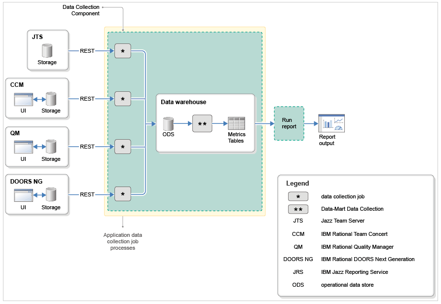

Figure 1. Reporting Architecture

Jazz Reporting Service get information from the Jazz Team Server (abbreviated JTS in the figure), IBM Rational Team Concert (CCM), IBM Rational Quality Manager (QM) and IBM Rational DOORS Next Generation (DOORS NG). The information is retrieved by the so-called Data Collection Components which serves as Extract-Transform-Load (ETL) jobs in this architecture. The information is loaded into the Operational Data Store (ODS) part of the the Data Warehouse first, and having passed this phase, other data collection jobs are responsible for filling the metric tables with data for trend reporting.

The Data Warehouse has 3 schema’s that are relevant for reporting:

RIODS (originally an abbreviation for Rational Insight Operational Data Store) that consist of highly normalized database tables containing information regarding the various CLM artefact’s such as projects, work items, requirements and test artefact’s – including their attributes and relationships.
RICALM (Rational Insight Collaborative Application Lifecycle Management) that contains information related to custom CLM attributes as well as history tables for reporting on artifact changes, such as changes to the requirements, work items and test cases (amongst others).
RIDW (originally an abbreviation for Rational Insight Data Warehouse) that contains information for the various data marts to support trend reporting. Basically this boils down to star schema’s being defined in terms of fact tables storing the metrics as well as the dimension tables representing the dimensions of the star schema.

The RIDW contains – in extend – a set of de-normalized views over the ODS tables, which come in handy for reporting purposes. The ODS basically provides a partial snapshot of the information in the CLM tools reflecting the state of affairs at the time where the data collection jobs were last run. The tables have a common structure and have been defined according to the same set of patterns. We shall look into this topic in the next section.

Simple Reporting over Data Warehouse Tables and Views

In this first report over the Data Warehouse we are interested in a pie chart showing the number of project areas according to their class (see Figure 2), i.e.the number of Rational Team Concert (RTC), Rational Quality Manager (RQM) and Rational Requirements Composer/Rational DOORS Next Generation projects (RRC).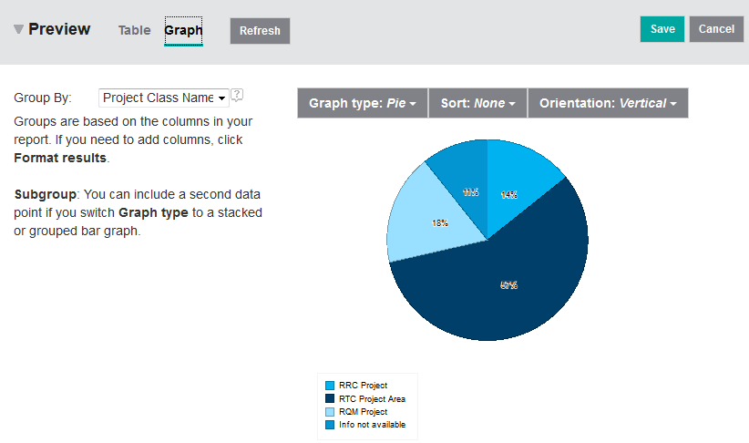

Figure 2. Pie chart showing project areas according to class

There are 3 basic steps involved in creating the report:

Understanding the underlying relevant data model of the Data Warehouse, i.e. where can you find the relevant data needed for the report.
Creating the relevant SQL statement.
Formatting the report so that it renders the data according to the reporting requirements.

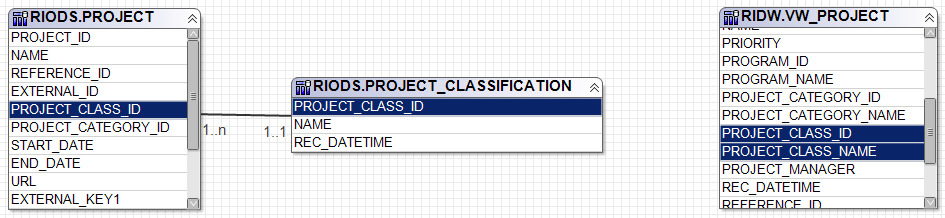
Lets start with the Data Warehouse first. What we need is a list of projects in the Data Warehouse together with some basic properties such as project name, project URL and of course the project class. There are two schema’s that contain such information in the Data Warehouse: the schema named RIODS and the schema named RIDW (See Figure 3). The advantage of using the schema RIDW as a basis for reporting rather than the schema RIODS is that the former offers a joined view (RIDW.VW_PROJECT) containing information from the table ODS.PROJECT as well as other tables such as RIODS.PROJECT_CLASSIFICATION (see Figure 3 for more details). Notice that view names are prefixed with VW_.

Figure 3. Data Warehouse tables and views for projects

The view gives direct access to the column PROJECT_CLASS_NAME which we need for the current reporting task. In contrast, the table RIODS.PROJECT is a basic table containing minimal information only, i.e. it contains the foreign key (PROJECT_CLASS_ID) but not the corresponding PROJECT_CLASS_NAME. The idea is that this information can be looked up if needed using the foreign key in the table RIODS.PROJECT_CLASSIFICATION. To keep things short: use views in the schema RIDW over tables in RIODS whenever you can because they contain more information relevant for reporting. This makes the second step – defining the SQL statement needed for the report – extremely simple in this case – and this is actually the whole reason why we have chosen this as the initial example for bare-bone Data Warehouse reporting (it will get more complicated later on):

SELECT	
	NAME,
	PROJECT_ID,
	REFERENCE_ID,
	URL,
	PROJECT_CLASS_ID,
	PROJECT_CLASS_NAME
FROM   RIDW.VW_PROJECT P
WHERE P.PROJECT_ID <> -1 AND P.ISSOFTDELETED = 0

In real life you may have to spend quite some time defining the SQL statement getting every detail right – it is usually an iterative process. You can use a variety of tools to support this. One option of course is the Jazz Reporting Service itself. Create a new report first and select e.g. Work Item as artifact. Then select Format Results, and finally select the Advanced tab, click Edit Query and delete the SQL statement that the query builder had created from the basis of the steps that you performed so far. You are now ready to put in your own SQL statement needed for defining the report (See Figure 4). Having entered the SQL statement you must validate it by clicking the Validate Query button:

SQL Query for retrieving project information

Figure 4. Enter and Validate Query

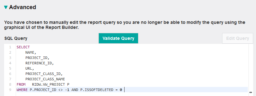
Validating the report will tell you whether the query is well-formed or not. However, it will not give you an idea whether the SQL statement has the right semantics – i.e. whether it returns the correct set of data or not. To test that the SQL statement is correct I usually render it as a Table first before I start changing the format to Graph. It therefore makes sense to complete the report definition and define proper labels for the columns. Then preview the report e.g. by clicking the Refresh button to check if the query returns the correct result (see Figure 5). Or even better – run the report to get the complete set of data returned by the SQL statement. Having checked that the SQL statement returns the correct data you must change the layout of the report from Table to Graph, select Pie as graph type and select the Project Class Name as the column to Group By (see Figure 2).

Figure 5. Query Preview

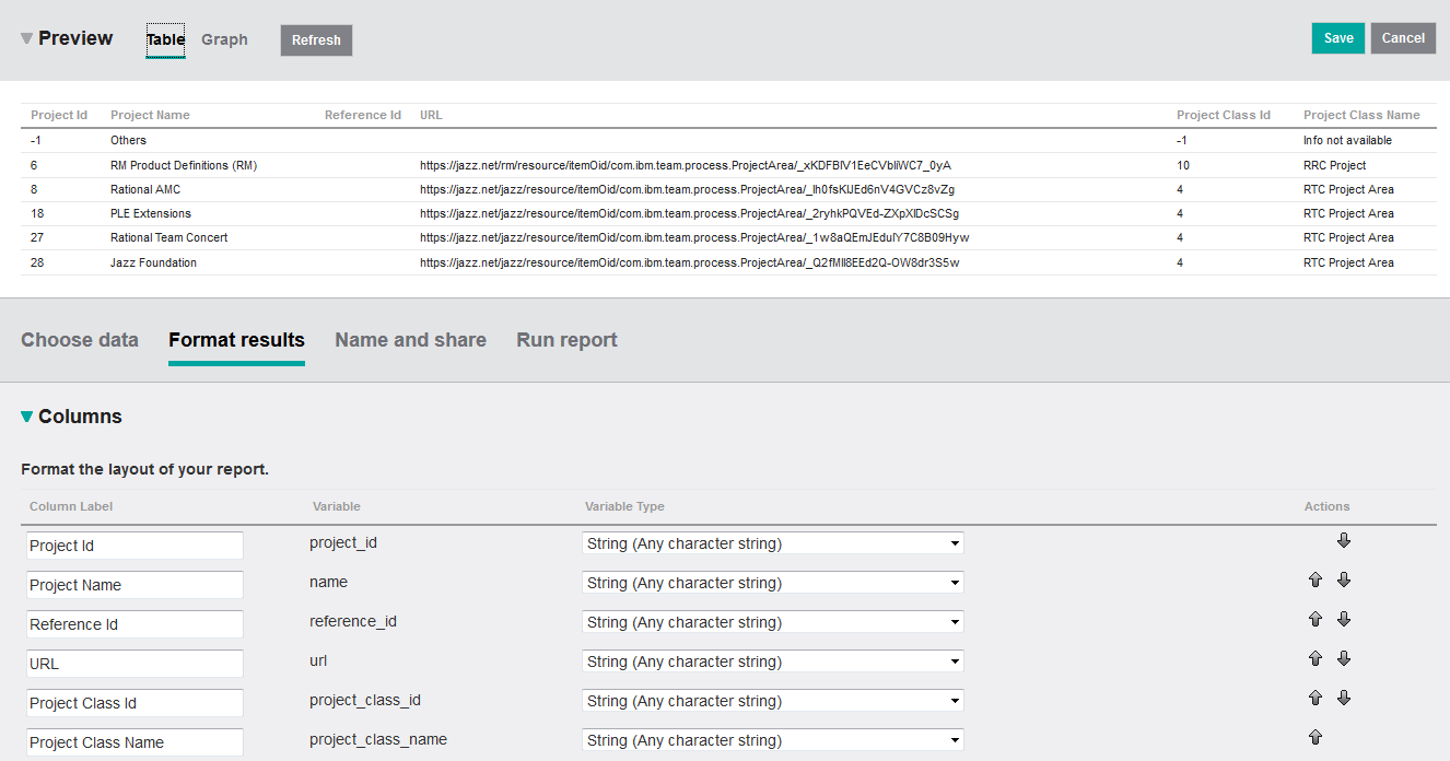
The simple query exposes some patterns that are found throughout the entire Data Warehouse. Many tables in the Data Warehouse are defined with a number of standard columns – some of which can be observed in the query that we have just defined (see Table 1 for a more complete list). For example, every PROJECT in the Data Warehouse has a unique internal identifier (PROJECT_ID). If you look at the first row of the results returned in Figure 5 you will observe that the first row has PROJECT_ID equal to -1. Many tables in the Data Warehouse got a predefined row with key -1. This value is used in foreign keys to designate the NULL pointer so to say, i.e. a PROJECT_CLASS_ID of -1 is used in a project that got no associated project class, a PROJECT_ID of -1 would be used to describe an entity that does not belong to a project. The corresponding name for such an entity is frequently the string “Info not available” – or in case of project simply the string “Others”.

Moreover, please observe that a row is never physically deleted in the Data Warehouse, rather the value of ISSOFTDELETED is changed from 0 to 1 when deletion in the source has occurred. In the Data Warehouse you will observe that there are other common columns used in many tables such as SOURCE_ID, EXTERNAL_KEY1, EXTERNAL_KEY2 and REC_DATETIME. These columns uniquely identify the entity upon re-import by the Data Collection jobs, and also gives information about the last import date.

Name	Explanation
PROJECT_ID	Unique internal key of type INTEGER which is automatically generated by the Data Collection Component when the corresponding row is inserted into a table the first time.
PROJECT_CLASS_ID	The foreign key that designates a specific entity in another table, in this case the table PROJECT_CLASS.
NAME	Contains the name of the entity, i.e.. the name of the project area or for work items the Summary.
REFERENCE_ID	Contains the identifier of the entity visible to the user. For work items it would be the integer number uniquely denoting the work item in a project area.
URL	The (Jazz) Uniform Resource Locater (URL) of the designated entity.
EXTERNAL_KEY1	An external (INTEGER) key for the entity, i.e. for work items the work item number.
EXTERNAL_KEY2	An external key in the form of a STRING.
SOURCE_ID	Identification of the source of the entity, i.e. the project area.
REC_DATETIME	The last date of import where the entity was changed
ISSOFTDELETED	An INTEGER that defines whether the entity is soft deleted (1) or not (0).

Table 1. Typical Columns used the Data Warehouse

Notice that bulk text such as descriptions and larger formatted text fields are not present in the Data Warehouse. In order to report on such information you will need to use e.g. the IBM Rational Publishing Engine for reporting using the Representational State Transfer (REST) services of the development tools.

Traceability Reporting using Lookup Tables and Derived Attributes

In this example we shall create a report that shows the test coverage of requirements , i.e. whether a requirement is covered by a test case or not. The preview of the report is shown in Figure 6.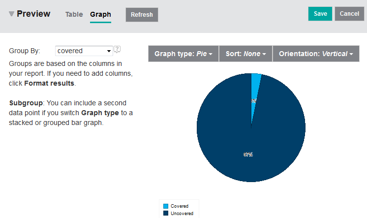

Figure 6. Requirement Test Coverage

As in the previous example there are 3 basic steps involved in creating the report: 1) understanding the underlying relevant data model of the Data Warehouse, 2) creating the required SQL statements and 3) formatting the report so that it renders the data as wished. For what concerns the first topic – the Data Warehouse tables or views to be precise – the information is stored in 2 relevant views in this case. A view RIDW.VW_REQUIREMENT gives information about the requirements whereas another view named RIDW.VW_REQUIREMENT_TESTCASE_LOOKUP defines a binary relationship defining the association of requirements to test cases. In other words, the so-called lookup table stores information related to the CLM “Validated By” links. Figure 8 gives an overview of the data model.

Data model for requirement traceability to test cases

Figure 7. Data Model for requirement test case lookup

You will find these lookup tables in many places in the Data Warehouse and they are used to define trace information due to e.g. OSLC links such as a trace from a requirement to a test case. Some of the lookup tables are also used to define the association between collections and their contained element, such as VW_REQUICOL_REQUIREMENT_LOOKUP that defines the relationships between requirement collections on the one hand and the contained requirements on the other. However you may also find tables in the Data Warehouse that have the suffix _HIERARCHY such as VW_REQUIREMENT_HIERARCHY. These tables are intended to present links between parent objects and child objects, e.g. from a parent requirement to a child requirement. They are similar in structure to the LOOKUP tables.

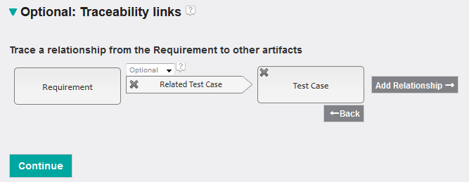
There is an easy way to get to a basis for the SQL statement that will be needed to define the report. You can simply create a new Jazz Reporting Service report, select Requirement as scope for the report and then select a trace to a test case:

Figure 8. Using the Query Builder to define the basis for the report

This will generate a SQL statement which will need to be changed to something that looks like:

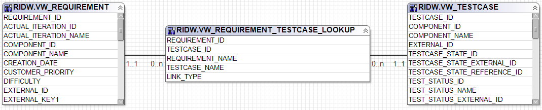
SELECT DISTINCT 
        T1.REQUIREMENT_ID,
        CASE   
              WHEN LT1.TESTCASE_ID IS NULL THEN 
                   'Uncovered'
              ELSE 'Covered'
        END  AS COVERED
FROM RIDW.VW_REQUIREMENT T1
LEFT OUTER JOIN RIDW.VW_REQUIREMENT_TESTCASE_LOOKUP LT1
ON T1.REQUIREMENT_ID = LT1.REQUIREMENT_ID
WHERE (T1.PROJECT_ID = 62) AND (T1.ISSOFTDELETED = 0)  AND (T1.REQUIREMENT_TYPE = 'CapabilityRequirement'))

The SQL statement takes its origin in the view VW_REQUIREMENT, and joins it with the view VW_REQUIREMENT_TESTCASE_LOOKUP to get the associated requirements and linked test cases. Notice that the join is an outer join meaning that it will still return a result row for a requirement even if the requirement has no matching test case. This is actually a minimal example in using lookup tables. All you would need to do now would be to paste this SQL statement into the report as the underlying query for the report, validate it and then re-order and rename the resulting columns. Notice that the output delivered by the query is kept to a minimum as well: it consists of just the requirement identifier followed by a computed column delivering an indication whether the requirement is covered by a test case or not.

By the way: in defining such queries I prefer working with internal Data Warehouse identifiers rather than REFERENCE_IDs since I know that the internal identifiers such as REQUIREMENT_ID are a) filled with data and b) unique. REFERENCE_IDs do not necessarily exhibit those properties. The REFERENCE_ID for a requirement for example is the requirement integer number as it is visible to the user in the user interface of IBM Rational DOORS Next Generation (e.g. 60). A requirement in another project area may of course have the same reference identifier. The internal identifiers are in contrast unique. The first requirement to be imported into the Data Warehouse will get REQUIREMENT_ID equal to 0, the next to 1 – so forth and so on.

The final step is to choose report layout. You should start by selecting Pie for the Graph type. Then set the Group By option to covered as shown in Figure 6.

Reporting over Custom CLM Attributes

Suppose that we would like to refine the report just defined so that it shows test coverage discriminating over some kind of custom requirement attribute like for example “Business Priority”. This will require the use of a stacked bar chart as shown in Figure 9.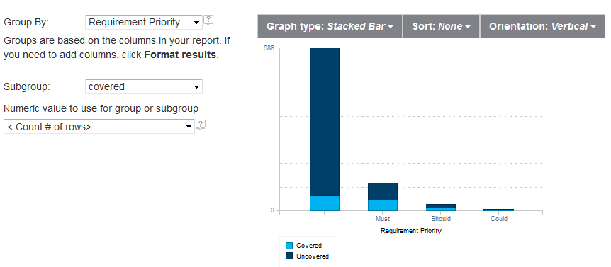

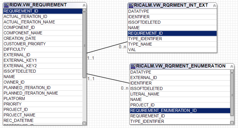
Figure 9. Requirement test coverage by requirement priority

Information regarding the custom CLM attributes are kept in the CALM schema of the Data Warehouse. As for the projects there are two kind of definitions: base normalized tables and views (that are more convenient for reporting). I shall focus on the views only. One example is the view RICALM.VW_RQRMENT_INT_EXT (standing for requirement integer extension) which, for enumeration attributes, stores a triple consisting of the internal REQUIREMENT_ID, custom attribute NAME and the integer value of the enumeration literal (VAL). Another relevant view is RICALM.VW_RQRMENT_ENUMERATION which provides the triple REQUIREMENT_ID, NAME, LITERAL_NAME which is exactly what is needed for reporting purposes over custom enumeration attributes. There are similar extension tables for booleans (BOOL), decimals (DECIMAL), strings (STRING) and dates (DATE).

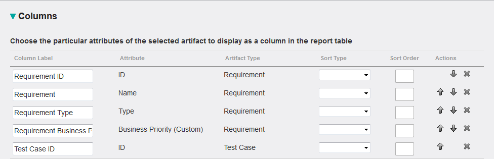
Figure 10. Data model for custom attributes

You can get to the basis of that report simply by using the query builder. Select requirement as the object in scope for the report, followed by the relevant attributes – including the custom attribute needed for the report (e.g. “Requirement Priority” or “Requirement Business Priority” say). Then define a trace to the test case as in the previous report.

Figure 11. Using the Query Builder to define the basis for the report

Next, the tell the query builder that you would like to edit the generated SQL statement and change the result columns to compute whether the requirement is covered by a test case or not:

SELECT DISTINCT 
       T1.REQUIREMENT_ID,
       T3.LITERAL_NAME,
        CASE   
              WHEN T2.REFERENCE_ID IS NULL THEN 
                   'Uncovered'
              ELSE 'Covered'
        END  AS COVERED
FROM RIDW.VW_REQUIREMENT T1
LEFT OUTER JOIN RIDW.VW_REQUIREMENT_TESTCASE_LOOKUP LT1
ON T1.REQUIREMENT_ID = LT1.REQUIREMENT_ID
  LEFT OUTER JOIN RIDW.VW_TESTCASE T2
  ON T2.TESTCASE_ID = LT1.TESTCASE_ID
      LEFT OUTER JOIN RICALM.VW_RQRMENT_ENUMERATION T3
      ON T3.REQUIREMENT_ID=T1.REQUIREMENT_ID AND T3.NAME='Business Priority'
WHERE ... filter on project id, requirement types etc

More complex traceability reports

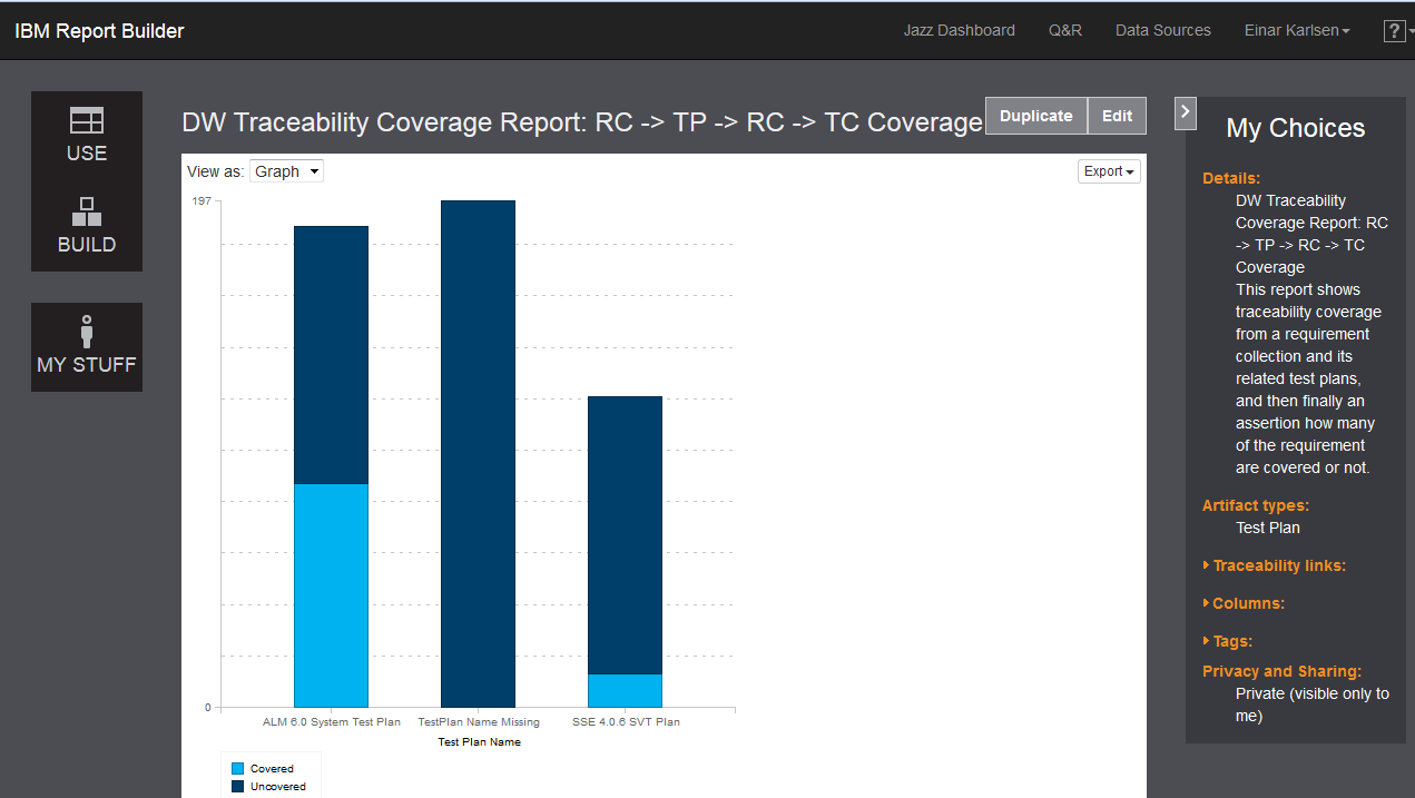
So far I have shown you reports with increasing level of complexity and at the same time introduced the key concepts of the underlying Data Warehouse one by one. I would like to end with a real life example coming from a system client. System clients are very much into traceability, and the report that the client requested was basically a report that should take its basis in requirement collections following traces to the relevant test plans, and then show the requirement coverage for each test plan. An example of the underlying list report can bee seen in Figure 11.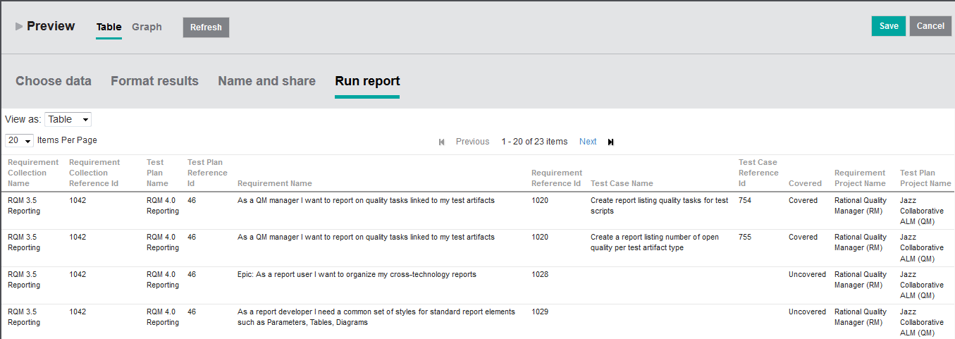

Figure 12. Traceability Report – basic data as a list

In fact, this report can’t be defined in a straight forward manner using the query builder of Jazz Reporting Service. Basically, the report requires that we compute 2 sub-queries that are then joined at the very end in a sort of “meet in the middle” approach. The first sub-query that is needed shows the traceability from test plans, over constituent test cases to linked requirements. This query is defined by the following SQL statement (lets call the query VW_TESTPLAN_TESTCASE_REQUIREMENT_LOOKUP in the following):

SELECT 
	TTL.TESTPLAN_ID,
	TTL.TESTPLAN_NAME,
	TTL.TESTCASE_ID,
	TTL.TESTCASE_NAME,
	RTCL.REQUIREMENT_ID,
	RTCL.REQUIREMENT_NAME
FROM   RIDW.VW_TESTPLAN_TESTCASE_LOOKUP TTL
LEFT OUTER JOIN   RIDW.VW_REQUIREMENT_TESTCASE_LOOKUP RTCL ON RTCL.TESTCASE_ID = TTL.TESTCASE_ID

The query uses two lookup tables: TESTPLAN_TESTCASE_LOOKUP to determine the relationship between test plans and its constituent test cases and the lookup table VW_REQUIREMENT_TESTCASE_LOOKUP that defines the links between requirements and test cases (and vice versa). The two views are joined together by comparing TESTCASE_IDs using an outer left join which means that it will also show the test cases for which there is no associated requirement at all.

The second sub-query defines the traceability from requirement collections, via test plans to the requirements of the requirement collection. This query can be defined by the following SQL statement (lets call that query VW_REQUICOL_TESTPLAN_REQUIREMENT_LOOKUP):

SELECT	
	RTL.REQUIREMENT_COLLECTION_ID,
	RTL.REQUIREMENT_COLLECTION_NAME,
	RTL.TESTPLAN_ID,
	RTL.TESTPLAN_NAME,
	RTL.LINK_TYPE,
       RRL.REQUIREMENT_ID,
       RRL.REQUIREMENT_NAME
FROM   RIDW.VW_REQUICOL_TESTPLAN_LOOKUP RTL
JOIN   RIDW.VW_REQUICOL_REQUIREMENT_LOOKUP RRL ON RRL.REQUIREMENT_COLLECTION_ID = RTL.REQUIREMENT_COLLECTION_ID

The final query defining the requested traceability is then defined as follows:

SELECT 
	RTRL.REQUIREMENT_COLLECTION_ID,
	RTRL.REQUIREMENT_COLLECTION_NAME,
	RTRL.TESTPLAN_ID,
	RTRL.TESTPLAN_NAME,
	RTRL.LINK_TYPE,
	RTRL.REQUIREMENT_ID,
	RTRL.REQUIREMENT_NAME,
	TTRL.TESTCASE_ID AS TESTCASE_ID,
	TTRL.TESTCASE_NAME,
        CASE   
              WHEN TTRL.TESTCASE_ID IS NULL THEN 'Uncovered'
              ELSE 'Covered'
        END  AS COVERED

FROM   (<VW_REQUICOL_TESTPLAN_REQUIREMENT_LOOKUP>) RTRL
LEFT OUTER JOIN (<VW_TESTPLAN_TESTCASE_REQUIREMENT_LOOKUP>) TTRL ON TTRL.TESTPLAN_ID = RTRL.TESTPLAN_ID AND TTRL.REQUIREMENT_ID = RTRL.REQUIREMENT_ID

Basically the query joins the two queries that we have previously defined by comparing TESTPLAN_IDs and REQUIREMENT_IDs. Lets call this query <TRACES> because it basically defines the rather complicated traceability relationships in this case with minimal information. It does so using internal Data Warehouse identifiers which can’t be used as a basis for rendering the report to a human being. The human reader may know the meaning of the REFERENCE_IDs or the URLs but can’t do much with the internal identifiers. So a last final step is needed joining the traces with the relevant base views for requirements, test plans and test cases in order to retrieve the more user friendly identifiers:

SELECT 
	TRACES.REQUIREMENT_COLLECTION_NAME,
   	RC.REFERENCE_ID AS REQUIREMENT_COLLECTION_REFERENCE_ID,
    	RC.PROJECT_NAME AS REQUIREMENT_PROJECT_NAME,
	TRACES.TESTPLAN_NAME,
    	TP.REFERENCE_ID AS TESTPLAN_REFERENCE_ID,
    	TP.PROJECT_NAME AS TESTPLAN_PROJECT_NAME,
	TRACES.REQUIREMENT_NAME,
    	RQ.REFERENCE_ID AS REQUIREMENT_REFERENCE_ID,
	TRACES.TESTCASE_NAME,
    	TC.REFERENCE_ID AS TESTCASE_REFERENCE_ID,
    	TRACES.COVERED
FROM(<TRACES>) TRACES
JOIN RIDW.VW_REQUIREMENT_COLLECTION RC ON RC.REQUIREMENT_COLLECTION_ID = TRACES.REQUIREMENT_COLLECTION_ID
JOIN RIDW.VW_TESTPLAN TP ON TP.TESTPLAN_ID = TRACES.TESTPLAN_ID
JOIN RIDW.VW_REQUIREMENT RQ ON RQ.REQUIREMENT_ID = TRACES.REQUIREMENT_ID
JOIN RIDW.VW_TESTCASE TC ON TC.TESTCASE_ID = TRACES.TESTCASE_ID

Following this exercise in defining complex SQL statements it is actually quite easy to perform a last step in order to render the information as a set of stacked bars showing the coverage of the requirements for each individual test plan involved.

Figure 13. Traceability Report showing requirement coverage as stacked bar chart

Conclusion

In this article I have shown you how to define more advanced reports over the Data Warehouse using SQL statements as a basis rather than the query builder – except in a few cases where the query builder can indeed be used to generate small fragments of the solution. At the same time – and this is almost more important – I have taken the opportunity to provide an overview of the Data Warehouse – its schema’s, tables, views, naming conventions and solution patterns. In order to get more familiar with the Data Warehouse I can only recommend to connect to the Data Warehouse using a local installation and then browse the catalog. A very helpful dictionary is furthermore available on the IBM Rational Knowledge center [IBM 2015].

The current article has a strong focus on reporting over the current state of affairs. A second article will appear later in 2015 showing how to use Jazz Reporting Service to define custom trend reports using SQL and history tables as well as the star schema’s available in the Data Warehouse. However, this will require use of v6 of CLM.

References

[Bater 2014] Robin Bater: Rational Reporting Made Simple: Using Out of the Box Reports, https://www.youtube.com/watch?v=DnCxavfFcLg, 2014.
[Haumer 2014] Peter Haumer: Discover cross-project reporting with the IBM Jazz Reporting Service, IBM Rational Software, https://jazz.net/library/article/1417, 2014.
[IBM 2014] IBM Rational User Education Service: IBM Rational Jazz Reporting Service, https://www.youtube.com/playlist?list=PLZGO0qYNSD4WC3zD9bQuejVSVofVLE9nq, 2014.
[IBM 2015] IBM Rational Knowledgecenter: Reporting Data Dictionaries, http://www-01.ibm.com/support/knowledgecenter/SSYMRC_5.0.2/com.ibm.rational.reporting.overview.doc/topics/c_reference_datadictionary.html?lang=en, 2015
[Shaw2014] Steven Shaw: Advanced Report Creation in Jazz Reporting Service 5.0.2, IBM Rational Software, https://jazz.net/library/article/1470, 2014.

About the authors

Dr. Einar Karlsen has been with Rational Software since 1998 supporting clients in the adoption of tools and methods for Requirement, Architecture and Test Management and is currently working as Solution Architect for Application Lifecycle Management solutions within the IBM Rational organization. He is currently Technical Lead for reporting within the IBM Rational organization in Germany.

Dashboards and work items are no longer publicly available, so some links may be invalid. We now provide similar information through other means. Learn more here.

Feedback

Was this information helpful?

Yes

No 9 people rated this as helpful.